e244824's blog

I have implemented procedural city generation on OpenGL and in this blog post, I will explain my implementation process and discuss my results.

My initial plan was to implement the following features:

• Procedural grid rendering using Wang Tiles and noise sampling.
• Building generation using L system grammars and level-of-detail rendering.
• Greenery generation using L system grammars and noise sampling.

In the sections below, I will explain my implementation process for each feature in detail.

Grid Generation

The purpose of generating a grid was to determine the contents of each tile in a manner that would look natural. To achieve this, my plan was to sample from a noise function to determine a few initial tiles, and then generate the rest of the grid by using Wang tiles with appropriate constraints or, if that produced unacceptable results, use Wave Function Collapse to generate the rest of the grid seamlessly.

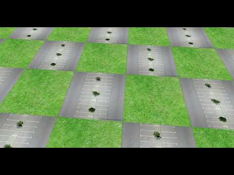
I initially planned on using Perlin noise through an existing library called ‘stb_perlin.h’. However, its perlin_noise3() function only generated values with very small absolute values (below 0.1 in most cases) for some reason, so I decided to implement the function myself. My first attempt was to utilize the function I used for my third homework in this course. For some reason, it produced a checker-like pattern. The video below shows a 10 by 10 grid that was generated by sampling from my Perlin noise function. To visualize the contents initially, I simply rendered some pictures for each main tile type (grasses for greenery, a straight road for the roads, and a parking lot for the buildings)

While looking for some resources on the technical details of Perlin noise, I came across this video. I decided to reimplement using this video as a guide, and my new function provided much better results:

For this implementation, I used 2D Perlin noise with the following gradient vectors:

const glm::vec2 gradients[8] = {
    glm::vec2(1, 0),
    glm::vec2(-1, 0),
    glm::vec2(0, 1),
    glm::vec2(0, -1),
    glm::vec2(1, 1),
    glm::vec2(-1, 1),
    glm::vec2(1, -1),
    glm::vec2(-1, -1)
};

The interpolation function for this implementation is different from the one on the course slides. Instead of using -6|x|⁵+15|x|⁴-10|x|³+1, it uses 6x⁵-15x⁴+10x³. Other than that, the implementation is mostly similar to the one on our course slides:

int hash(int x, int y) {
    return (((x % 256) + y) % 256) % 8;
}


float fade(float t) {
    return t * t * t * (t * (t * 6 - 15) + 10);
}


float lerp(float a, float b, float t) {
    return a + t * (b - a);
}


float dotGridGradient(int ix, int iy, float x, float y) {
    glm::vec2 gradient = gradients[hash(ix, iy)];
    float dx = x - (float)ix;
    float dy = y - (float)iy;
    return (dx * gradient.x + dy * gradient.y);
}


float perlin(float x, float y) {
    // Determine grid cell coordinates
    int x0 = (int)floor(x);
    int x1 = x0 + 1;
    int y0 = (int)floor(y);
    int y1 = y0 + 1;

    // Determine interpolation weights
    float sx = fade(x - (float)x0);
    float sy = fade(y - (float)y0);

    // Interpolate between grid point gradients
    float n0, n1, ix0, ix1, value;

    n0 = dotGridGradient(x0, y0, x, y);
    n1 = dotGridGradient(x1, y0, x, y);
    ix0 = lerp(n0, n1, sx);

    n0 = dotGridGradient(x0, y1, x, y);
    n1 = dotGridGradient(x1, y1, x, y);
    ix1 = lerp(n0, n1, sx);

    value = lerp(ix0, ix1, sy);

    //return (value + 1) / 2;
    return abs(value);
}

To map the values between 0 and 1 I tried both (n(x,y)+1)/2 and |n(x,y)|. From the tests I’ve done, the second option seemed to yield better results, but this mostly depends on how one maps the tile values to the noise values.

Once I increased the grid size and changed the mapping a bit, I got the following pattern:

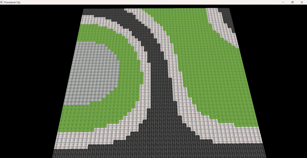
The black tiles represent roads, the green tiles represent the greenery, and the greyish tiles that are clumped together represent the building tiles. This produced quite a nice pattern in my opinion. So I increased the size to 100 by 100 and tweaked the mapping just a bit more to produce this pattern:

This pattern looks quite nice in my opinion. The building blocks are grouped together, which should lead to more buildings being generated near each other with greenery tiles between building clusters. I should mention that I used the gradient vectors without random indexing or creating random gradient vectors, so the Perlin noise map is constant. This is fine though, as my plan is to just sample some initial tiles and then start generating from those tiles according to their constraints, leading to varying but consistent patterns. At least, that was my plan.

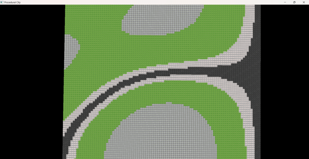
Once that was done, I tried to add some constraints and generate the tiles according to them. Below are two 25 by 25 grids where the first one was created with 5 samples and the second one was created with 25 samples:

While more samples lead to more variance, the overall pattern looked quite randomized. The reason behind this is my constraints being inadequate. I tried to improve the pattern by adding more tile types and different constraints further on but I couldn’t achieve a good looking pattern.

Tree Generation

To generate trees, I utilized an L system grammar. I was initially also going to sample from a noise function to determine the positions of trees within a tile, but since the tiles were already quite small and the buildings were going to be scaled according to the tiles, I decided to render one tree per greenery tile, and determine the type of tree at that tile by sampling from the mapped Perlin noise values.

The L system I used for the trees works as follows:

Forward (‘F’):

• Calculate the next position by moving forward.
• Add a cylinder segment.
• Update the current position.

Rotate Right (‘+’):

• Rotate by 25 degrees around the Z-axis in a positive direction.

Rotate Left (‘-‘):

• Rotate by 25 degrees around the Z-axis in a negative direction.

Push State (‘[‘):

• Push the current transformation matrix onto the stack.
• Push the current position onto the stack.
• Push the current thickness (as a scale matrix) onto the stack.

Pop State (‘]’):

• Pop the thickness from the stack and update thickness.
• Pop the current position from the stack and update current position.
• Pop the current transformation matrix from the stack and update the current matrix.

Below is the code for this system:

void parseLSystem(const std::string& lSystemString, std::vector<glm::vec3>& vertices, const glm::vec3& startPosition) {
    std::stack<glm::mat4> stack;
    glm::mat4 currentMatrix = glm::translate(glm::mat4(1.0f), startPosition);
    glm::vec3 currentPosition = startPosition;
    glm::vec3 forwardVector(0.0f, 0.5f, 0.0f); // Determines the length over a direction

    float initialThickness = 0.09f;
    float thickness = initialThickness;

    for (char c : lSystemString) {
        if (c == 'F') {
            glm::vec3 nextPosition = currentPosition + glm::vec3(currentMatrix * glm::vec4(forwardVector, 0.0f));
            addCylinderSegment(vertices, currentPosition, nextPosition, thickness);
            currentPosition = nextPosition;
        }
        else if (c == '+') {
            currentMatrix = glm::rotate(currentMatrix, glm::radians(25.0f), glm::vec3(0.0f, 0.0f, 1.0f));
        }
        else if (c == '-') {
            currentMatrix = glm::rotate(currentMatrix, glm::radians(-25.0f), glm::vec3(0.0f, 0.0f, 1.0f));
        }
        else if (c == '[') {
            stack.push(currentMatrix);
            stack.push(glm::translate(glm::mat4(1.0f), currentPosition));
            stack.push(glm::scale(glm::mat4(1.0f), glm::vec3(thickness)));
        }
        else if (c == ']') {
            thickness = glm::scale(stack.top(), glm::vec3(1.0f, 1.0f, 1.0f))[0][0];
            stack.pop();
            currentPosition = glm::vec3(stack.top()[3]);
            stack.pop();
            currentMatrix = stack.top();
            stack.pop();
        }
        thickness *= 0.8f; // Reduce the thickness for the next segment
    }
}

By using this system, I generated 6 different tree structures with different strings. Below are the outputs of each string.

Basic branching tree (“F[+F]F[-F]F”):

Dense branching tree (“F[+F[+F]F[-F]]F[-F[+F][-F]F]”):

Somewhat symmetrical tree (“F[+F[+F]F[-F]]F[-F[+F]F]F[+F]F[-F]”):

Wide spread tree: (“F[+F[+F[+F]F[-F]]F[-F[+F]F[-F]]]F[-F[+F]F[-F[+F]F[-F]]]F[+F]F[-F]”):

High complexity tree (“F[+F[+F[+F]F[-F]]F[-F[+F]F[-F]]]F[-F[+F[+F]F[-F]]F[-F[+F]F[-F]]]F[+F[+F[+F]F[-F]]F[-F[+F]F[-F]]]F[-F]”):

Bifurcating tree (“F[+F[+F]F[-F]]F[-F[+F]F[-F[+F]F[-F]]]F[+F[+F]F[-F]]”):

And below is trees being generated on a 25 by 25 grid:

I was going to implement a function to generate several random tree strings according to the L system rules, but I didn’t have enough time to implement it (I couldn’t even render some leaves for the trees).

Building Generation

To generate the buildings, I again used L system grammars. The building grammar is quite simple:

Wall (‘F’):

• Add a wall segment from current position to next position.
• Rotate by -90 degrees for the next segment.

Window (‘W’):

• Similar to ‘F’, but adds a window segment instead of a wall.

Door (‘D’):

• Similar to ‘F’, but adds a door segment instead of a wall.

Roof (‘R’):

• Add a roof from the current position.

Move Up (‘+’):

• Move upwards by height. Basically creates a new floor.

And here’s the code for the system:

void parseBuildingLSystem(const std::string& lSystemString, std::vector<glm::vec3>& vertices, const glm::vec3& startPosition) {
    std::stack<glm::mat4> stack;
    glm::mat4 currentMatrix = glm::translate(glm::mat4(1.0f), startPosition);
    glm::vec3 currentPosition = startPosition;
    glm::vec3 forwardVector(1.0f, 0.0f, 0.0f); // Forward vector for building segments

    for (char c : lSystemString) {
        if (c == 'F') {
            glm::vec3 nextPosition = currentPosition + glm::vec3(currentMatrix * glm::vec4(forwardVector, 0.0f));
            addBuildingSegment(vertices, currentPosition, nextPosition, WALL);
            currentPosition = nextPosition;
            currentMatrix = glm::rotate(currentMatrix, glm::radians(-90.0f), glm::vec3(0.0f, 1.0f, 0.0f));
        }
        else if (c == 'W') {
            glm::vec3 nextPosition = currentPosition + glm::vec3(currentMatrix * glm::vec4(forwardVector, 0.0f));
            addBuildingSegment(vertices, currentPosition, nextPosition, WINDOW);
            currentPosition = nextPosition;
            currentMatrix = glm::rotate(currentMatrix, glm::radians(-90.0f), glm::vec3(0.0f, 1.0f, 0.0f));
        }
        else if (c == 'D') {
            glm::vec3 nextPosition = currentPosition + glm::vec3(currentMatrix * glm::vec4(forwardVector, 0.0f));
            addBuildingSegment(vertices, currentPosition, nextPosition, DOOR);
            currentPosition = nextPosition;
            currentMatrix = glm::rotate(currentMatrix, glm::radians(-90.0f), glm::vec3(0.0f, 1.0f, 0.0f));
        }
        else if (c == 'R') {
            glm::vec3 nextPosition = currentPosition + glm::vec3(currentMatrix * glm::vec4(forwardVector, 0.0f));
            addBuildingSegment(vertices, currentPosition, nextPosition, ROOF);
        }
        else if (c == '+') {
            currentPosition += glm::vec3(0.0f, 1.0f, 0.0f);
        }
    }
}

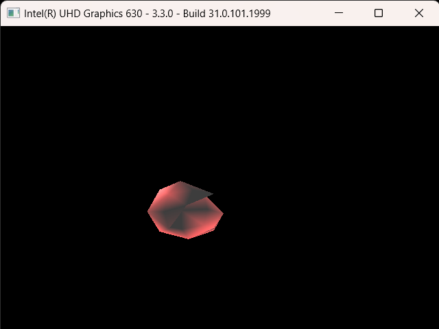
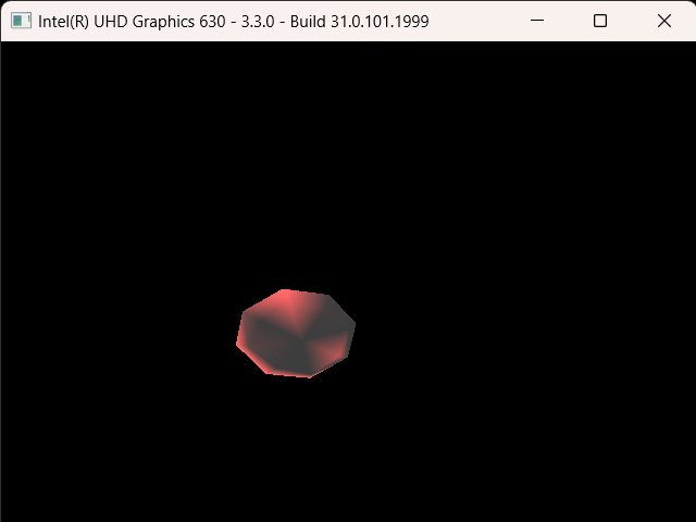
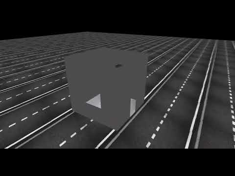
This system builds very simple buildings with randomized walls that either have a window or not. The ground floor also has a wall with a door in it. The video below showcases a simple building with a door, two windows, and a wall:

For the buildings, at least, I managed to implement a string generator that randomly generates building strings up to a given height (might be shorter). My implementation randomly generates 5 strings and renders the building from those models. Below is the implementation for it:

std::unordered_map> buildingRules = {
{‘F’, {‘F’, ‘W’}},
{‘W’, {‘F’, ‘W’}},
{‘D’, {‘F’, ‘W’}},
{‘+’, {‘F’, ‘W’, ‘R’}}
};

std::string generateBuildingString(int maxHeight = 3) {
std::string buildingString = “D”;
char lastChar = ‘D’;
int wallCount = 1, currentHeight = 0, constraintCount;

//std::cout << "Entered function\n";
while (currentHeight < maxHeight) {
    //std::cout << "Current string: " << buildingString << "\n";
    constraintCount = buildingRules[lastChar].size();
    char newChar = buildingRules[lastChar][rand() % constraintCount];

    if (newChar == 'F' || newChar == 'W' || newChar == 'D') {
        wallCount++;
    }

    buildingString += newChar;

    if (newChar == 'R') break;

    if (wallCount >= 4) {
        buildingString += '+';
        wallCount = 0;
        currentHeight++;
        lastChar = '+';
    }
    else {
        lastChar = newChar;
    }
}

return buildingString;

}

Unfortunately, I didn’t have much time to write a complex system, I barely had time to create the meshes for the walls and doors and windows.

This basically sums up my implementation. Here’s my final runtime video:

Final Discussions

Unfortunately, my implementation is admittedly very shoddy. I was originally supposed to implement this on Vulkan, but I just couldn’t grasp how Vulkan worked and just wasted most of my time. This is terrible time management on my part, as I’m sure I could have implemented something more concrete with interesting results. I could have tried randomizing the Perlin noise gradients and compare grids generated by Wang tile implementation and pure noise sampling. The trees could be rendered with more complex systems to generate some interesting models. Similarly, buildings could also be rendered in much more varying structure and actual texture instead of plain grey. Moreover, because the buildings had such simple meshes, I couldn’t really simplify the models further for LOD rendering. I even had to design the road textures by hand, yet some of them are rendered in red and I have no idea why. Still, I feel like I’ve learned quite a bit and I’d like to further develop this project in my spare time.

For my third homework as part of the Computer Graphics 2 course, I implemented grass rendering in OpenGL using the geometry shader, Bezier curves, and Perlin noise. In this blog post, I will explain my process of learning and implementing this homework.

Learning More About OpenGL

Before I started implementing this homework, I thought that it might be better if I first had a better grasp on how geometry shaders worked so I took a look at various tutorials on geometry shaders and found some interesting sources. While this section is not really important, I found some sources that I thought were really cool and I just wanted to share them somehow.

While looking through some posts on Reddit, I found a comment under this post suggesting a webpage called The Book of Shaders by  Patricio Gonzalez Vivo & Jen Lowe. It is an interactive website that explains how shaders work in detail, showcases some shaders and their results, and even allows you to rewrite those shaders and display your results in real-time. Below is a little sample shader in the “Uniforms” section that displays a flashing animation:

I also found a blog post called Bezier Curves and Picasso by Jeremy Kun where he explains the process in which he draws Pablo Picasso’s drawing called “Dog” using only Bezier curves. It also has an interactive demo that allows you to edit the control points of each curve, leading to some interesting results:

I understand that the sources I talked about above aren’t really related to the homework. I’ll start explaining my implementation process in the section below.

Grass Rendering Implementation

To implement the grasses, I decided to first randomly generate 1000 grasses with random x and z values with 3 control points, then sample the wind value from a temporary function that oscillates with time, and set the control point values from the geometry shader. I first rendered a bunch of simple green-colored line strips:

I though this was a decent starting point. Even with three control points the grasses looked decent enough. But I only implemented this as a starting point, I’m aware that these are not Bezier curves. I used the function below to generate some oscillating values with time:

float getWindVelocity(float x, float y, float time) {
    return 0.1 * cos(0.1 * x + time*2.0) * sin(0.1 * y + time*2.0);
}

I made use of ChatGPT to generate this function since this was supposed to be just a placeholder for the actual Perlin noise implementation (or so I thought at the time).

After this, I decided to implement the wind speed increase/decrease functionality, which was quite simple. I simply scaled the time variable with a variable that changed with input in the sampling function. Later on, I decided to scale the entire output instead, as it provided smoother swaying motions. In the demonstration below, I utilized the former version:

At this point, I needed to test my implementations with more grass blades that were spread over a larger area, but not all of the grasses were visible. So before I proceeded further with the main implementation, I added camera movements and rotations. The movement part was rather simple, to go forward or backward, simply updated the position by multiplying the Front vector with the speed value I set and added it to the position. To go left or right, I calculated the left and right vectors by taking the cross products of the Up and Front vectors.
The rotation part was a bit trickier. I was initially planning on using quaternions as was showcased in one of our lectures, but I couldn’t get a good grasp on the mechanism and I didn’t have much time, so I went for a simpler solution. I simply calculated the offset from the previous position, incremented the yaw and pitch values with the offsets (making sure that the pitch degree didn’t go over 89 degrees or below -89 degrees), and updated the Front and Up vectors with these values. Below is the implementation:

void mouse_callback(GLFWwindow* window, double xpos, double ypos) {
    if (firstMouse) {
        lastX = xpos;
        lastY = ypos;
        firstMouse = false;
    }

    float xoffset = xpos - lastX;
    float yoffset = lastY - ypos; // Reversed since y-coordinates range from bottom to top
    lastX = xpos;
    lastY = ypos;

    xoffset *= sensitivity;
    yoffset *= sensitivity;

    yaw += xoffset;
    pitch += yoffset;

    // Constrain the pitch
    if (pitch > 89.0f)
        pitch = 89.0f;
    if (pitch < -89.0f)
        pitch = -89.0f;

    glm::vec3 front;
    front.x = cos(glm::radians(yaw)) * cos(glm::radians(pitch));
    front.y = sin(glm::radians(pitch));
    front.z = sin(glm::radians(yaw)) * cos(glm::radians(pitch));
    cameraFront = glm::normalize(front);
}

And here is how it looks:

I was first going to implement the rotation by clicking and dragging on the screen so that the user could resize the window, or make it fullscreen. But unfortunately, I couldn’t really figure it out and I didn’t have much time left, so I had to move on. If resizing is absolutely necessary, the glfwSetInputMode at line 463 could be set to GLFW_CURSOR_NORMAL instead of GLFW_CURSOR_DISABLED. This would prevent the camera from being able to rotate completely because when the mouse reenters the window, the camera gaze starts from the initial position (I’m not sure why). By making the window fullscreen, you can rotate and move around enough to see the entire field.

Now I needed to render the blades as actual Bezier curves. I implemented the Bezier curves by first assigning four equally spaced control points to each grass blade starting from the ground coordinate to the assigned height value. Then, I interpolated 10 vertices between the starting point and the ending point using the functions in the course slides. When I rendered the grasses using triangle strips, I increased the amount to 21 segments. Below is how it looks:

I then rendered the grasses using triangle strips. This part was rather simple as well, I just rendered each segment using 2 vertices that went narrower as it grew higher. Since the deadline is technically not over yet and this is potentially an important part of the homework, I won’t post the implementation itself but here’s how it looks:

Now it was time to implement the keyboard functionalities requested as part of the homework. For changing colors, I made it so that the colors of the grasses rotated between three constant RGB values (green, yellow, white). Because not much was specified for this part, I didn’t waste too much time with it. I also added a ground mesh for a bit more aesthetic, but it didn’t really help much:

I decided to change the heights of the grasses between five values where each time the height is increased, it is scaled by 1.5 and vice versa. In terms of implementation, not much was needed since most of the processing was done on the geometry shaders. I just needed to change the stored grass blade data and reupload it to the VBO. I also decided to add some variance to the starting heights of the grasses to give it a more natural look. Here’s how it looks:

Finally, it was time to implement the Perlin noise functionality I had been procrastinating. Implementing the noise function itself wouldn’t be much of a problem, but I didn’t really know how I should sample from it as time went on. I first implemented the Perlin noise inside the geometry shader using the definitions given in the course slides yet again. While I first planned on implementing it using 2D coordinates, the slide specified that the 3D positions should be used to sample from the noise, so I simply went along with it. In hindsight, it was probably for grass field implementations that were done on a non-level surface (unlike mine), so perhaps my implementation would have looked a bit better if I used 2D coordinates but I’m not really sure. The demonstration below shows the grasses sampling from the first version of my Perlin noise implementation where I tried to add some dependency on time with a simple sin function, wind *= sin(time * windMult):

This result was quite unacceptable, but I didn’t really get a sense of how I could fix this. I realized the blades would bend one way while swaying the other, so I scaled the sampling down a bit at the lower parts of the blade. While this did fix the bending issue, the overall swaying animation looked way too stiff even if I capped the amount of swaying at a certain level.
As I was out of both ideas and time, I decided to utilize my so-called ‘temporary’ sampling function again to create a more natural-looking animation. It’s not that I didn’t use my Perlin noise implementation; I did, but instead of the coordinates, I passed the sampled noise values to the oscillating function. The outcome was serviceable, but obviously there is still much that could be done:

I also did some fps calculations on my own computer for the final version (fps was capped at 60 on the ineks):

	FPS (Window mode)	FPS (Fullscreen)
10,000 blades	950-1000	350
20,000 blades	500	200-250
40,000 blades	300	150-170
80,000 blades over larger area	250	90-120

And here’s a guide on the controls of the scene just in case. I have also added the guide in the readme file:

Q: Close the scene.

A/D: Increase/Decrease the wind speed. (0 to 3)

W/S: Increase/Decrease the grass blade length (0 to 4)

E/R: Cycle through the grass colors.

Arrow Keys: Camera movement.

This concludes my grass rendering implementation on OpenGL using Bezier curves, geometry shaders, and Perlin noise. While the base requirements have been met, there are still many features that could be added (skybox, non-level ground distribution) and areas that could be improved further (noise sampling, shading of the grasses). But, I still learned quite a bit from this assignment.

Welcome to my blog page. For my first assignment in the Computer Graphics 2 course, I implemented the Catmull-Clark Subdivision Surface algorithm, and in this post, I will be explaining my process of implementing this algorithm and the errors I encountered along the way.

To understand how the algorithm worked, I first tried to go over the paper “Recursively generated B-spline surfaces on arbitrary topology meshes” by E. Catmull and J. Clark, and the algorithm’s Wikipedia page. I also found a video that gives a simple step-by-step explanation of the algorithm, which helped clear up some parts I didn’t quite understand in the first two sources I mentioned. You can access the video through the following link: https://youtu.be/mfp1Z1mBClc?si=3LienRGDQvvMI0ht

Once I had a clear understanding of the algorithm, I started on my implementation. My initial thought was that it would be better to first write the algorithm itself. Once that was done, I could take care of the rest of the specifications given in the homework document (which was a mistake in hindsight), so I started writing a function on the sample code provided by the assistants.

Throughout writing my implementation, the main problem has always been calculating the vertex normals properly. Once my first implementation was done, I added an octahedron object and tested it. Below is the output:

The reason my output was like this was I believe because I forgot to add the newly calculated faces, but I’m not too certain. It was a minor mistake I had made and I fixed it relatively quickly. The main issues started after I fixed this issue.

Above are the outputs when the subdivision is applied once and then twice, in order. At first glance, I thought that maybe my algorithm was completely wrong, but I realized that the positions of the vertices seemed to be correct. Moreover, it seemed like for every new face I created half of it would not properly render. Since I had separated each new face into two triangles, I was most likely calculating the normal values incorrectly. Unfortunately, no matter what I did I could not fix this issue.

I was calculating the normals by first calculating the vectors going from the new face point to the edges and the corner. For example, let’s say that the new face I was calculating contained a new face point f, two edge points e1 and e2 that neighbored this face point, and a newly calculated vertex p that was between these two edges. I calculated three vectors: one from point f to point e1 (fe1), another from point f to point p (fp), and a third from point f to point e2 (fe2). Next, I computed the cross-products of the vectors fp and fe1, as well as fe2 and fp. Finally, I took the average of these cross-products and added their values to the normals of these vertices.
As one can tell from the results above, there was something wrong with this process. But as I mentioned before, the positions of the new vertices were, at least seemingly, correct, so there had to be something wrong with my normal calculation, at least that is the only possibility that came to my mind. I tried to switch the ordering when doing the cross-products, and the correctly rendered and incorrectly rendered faces seemed to switch. But for some reason when I kept one of the cross-product operations as it was, the entire object was incorrectly rendered.
I tried various other methods from taking the average of all of the normals of faces that were adjacent to a vertex to rewriting the entire function from scratch, but nothing I tried managed to fix this issue. Unfortunately by this point, I was running out of time, and I still had a lot to do so I decided to move on and maybe take a look again once everything else was done.

For the given assignment, I had to prepare a scene with multiple objects that were doing various movements. I decided to keep it simple and decided that I would add four objects, two of which would move perpendicular to each other and cross paths, and the other two would spin around themselves at opposite corners. It initially looked as it did below, with only an octahedron and a tetrahedron moving perpendicularly to each other:

To render multiple objects with their own vertex and fragment shaders, I used the model class my homework partner and I utilized for our final assignment in the Computer Graphics 1 course. I also had to implement a line mode and a wire mode visualization, which were relatively simple to make. The only issue was that there was some aliasing when the visualization was switched to line mode, and changing the glPolygonOffset did not help. As a small workaround, I instead increased the line width very slightly when drawing in line mode. Below is the visualization of line mode with aliasing:

And below is the version with fixed aliasing:

Once that was done, I implemented the functionality to decrease the subdivision level of the objects. Perhaps this might not be the most optimal solution in terms of memory, but I decided that it would be best to simply store the vertex, face, texture, and normal values of each object at each calculated level and simply reuse them when the subdivision level is decreased or re-increased. I understand that this solution might not translate well to a real-life scenario but since the subdivision operation would only be applied a maximum of four times per object, and my subdivision function was very inefficient, I believed that this would be the best solution.
Now, of course, there was a slight issue initially. When I first implemented this, most of the vertices would disappear when the subdivision level was decreased. By this point, I was a bit sleep-deprived so this situation left me a bit perplexed. The video below shows this error:

When I observed this error with a clearer head, I noticed something important: the remaining vertex count when decreasing the subdivision level is actually the amount it was supposed to be at that level, it was just the information of the vertices, faces, and whatnot that was not being updated. Then it dawned on me.

I had forgotten to re-initialize the models after decreasing the levels.

To say this infuriated me would be an understatement as it took an embarrassingly long time to figure this out, which left me with very little time, and I still had to go over my subdivision implementation again. Luckily I at least managed to finish the rest of the requirements. I think.
Below is how it is actually supposed to look. I also added some shading and a new object to the scene:

As I said before, I had decided that my scene would contain 4 objects, yet I’ve only shown 3 so far. The last one is the cube that I had to include in my scene as an obligation of the assignment. But what I had not known was that this cube consisted of quads instead of triangles. Now, this was actually mentioned to us during the briefing of the assignment, I think, but I had forgotten and had failed to properly read the assignment document, which also mentioned that there would be quad topologies (perhaps I’m legally blind).
Realizing this, I quickly started rewriting my parser function so that it could also parse quad objects. I achieved this by dividing each quad into two triangles and writing them to the buffers. I also kept the information of the quads so that I could use them when calculating the subdivision of the cube.
Below is the scene with the cube added:

Finally, I rewrote the subdivision function so that it could also work on quad topology. Unfortunately, my normal calculations were, again, incorrect so the cube was rendered incorrectly yet again.
Below is a video showcasing the final version of my program:

By this point, I barely had any time so I submitted my homework in this state. There were many things I could have improved, or properly implemented, but I mismanaged my time and underestimated the time needed to complete this homework. But still, I believe it is decent enough for homework that was done in three days, at least considering my own capabilities.