e244824's blog

For the third homework of my CENG 795: Advanced Ray Tracing course, I expanded my ray tracer by implementing multisampling using stratified random sampling, depth of field, motion blur, and glossy reflections. I also fixed the broken features, like my BVH implementation, and added the missing ones: PLY parsing and mesh instances. I will be explaining my implementation process and the problems I encountered along the way in this blog post.

Fixing the BVH Structure and Adding the Missing Features

The features I failed to implement in my previous homework were absolutely necessary for this homework, so I had to go over my implementation yet again and hope that I’d be able to properly implement those features this time otherwise I wouldn’t even be able to start this homework.

For the BVH, I decided to redo it from scratch, but I didn’t really change its overall logic. The biggest change I made was removing the bottom layer BVH structures for meshes and instead treating the mesh faces as primitives themselves. A 2 level BVH structure probably would have been faster, but a BVH that actually works is much faster than one that doesn’t work at all. For the traversal, I used stacks for depth first traversal and kept the maximum primitive count per leaf to 4. This implementation seemed to have worked, but I could only check on simple scenes without PLY meshes, so I had to implement the PLY parsing before I could completely be sure that it worked.

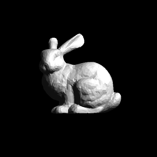
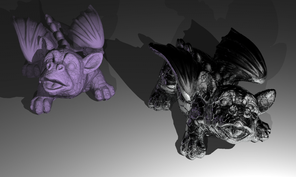
After I managed to compile the PLY library without a million issues, I encountered yet another problem! Even though I didn’t get any compilation errors, now the reader function gave errors whenever it tried to read an element in the file. The only exception was dragon_remeshed_fixed.ply, for some reason it could only read the contents of this file. At least that meant that the parser was working, it just couldn’t read some files for some reason. Every time I tried to run it on another file, it gave out this error: “get_binary_item: bad type = 0”. Seeing that it had problems reading some binary items, I tried converting the files to ASCII encoding and reading them that way. Thankfully this worked. If it hadn’t, I have no idea what I would have done. With that out of the way implementing mesh instances was quite simple, I had implemented the BVH with mesh instances in consideration.

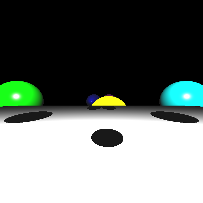
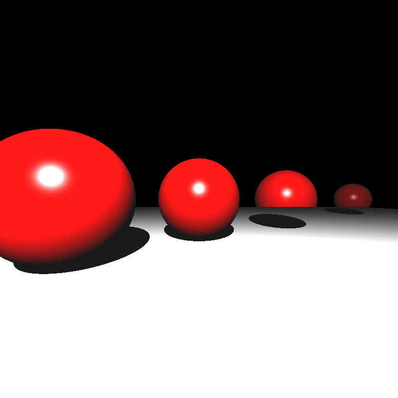
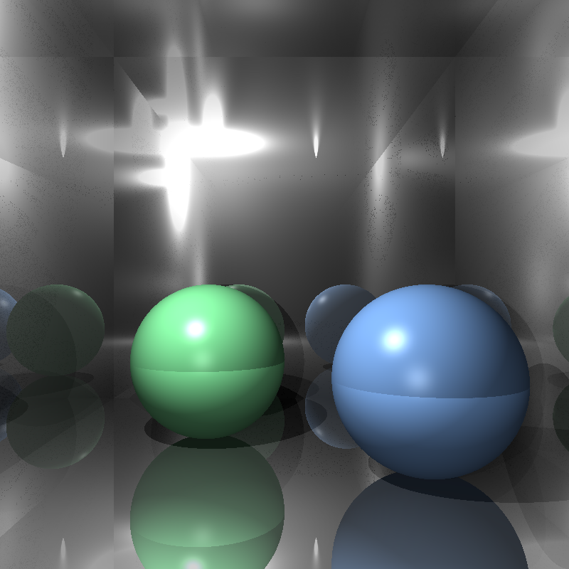
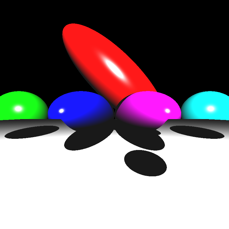
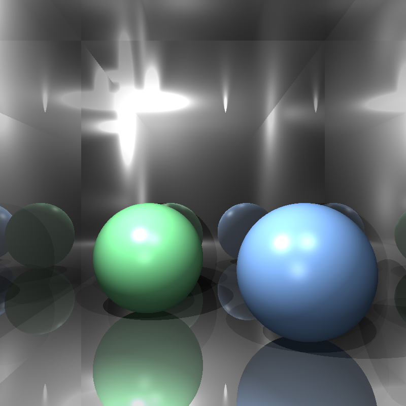
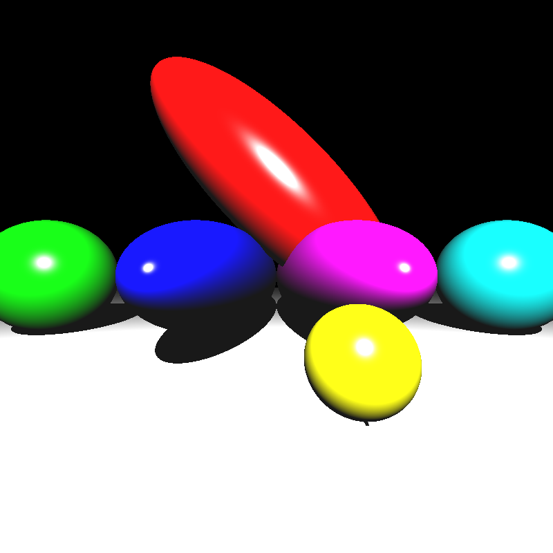
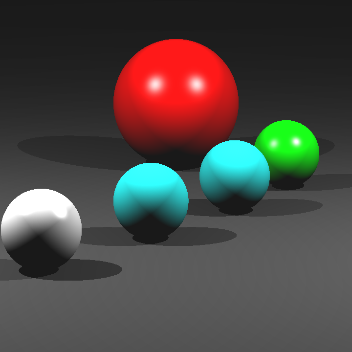
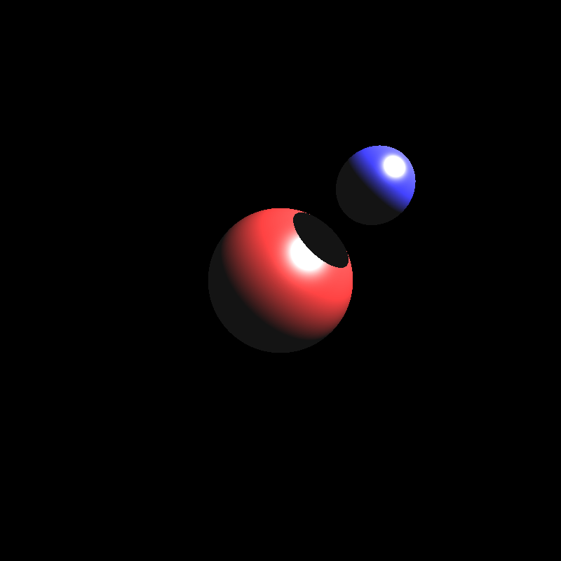
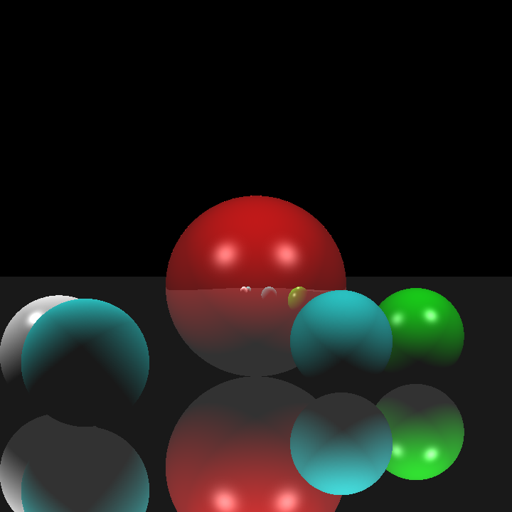
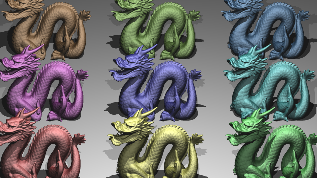
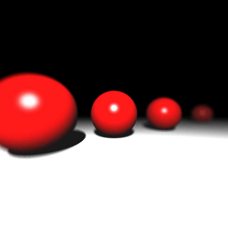
Now that all three features were implemented; I tested them, fixed some minor bugs I encountered, and finally I had a ray tracer that could read PLY files and had a working acceleration structure! Third time’s the charm I suppose. Below are the render times and the resulting images that were missing from my previous homework:

Scene File	Render Time (seconds)
ellipsoids.json	0.39
spheres.json	0.29
mirror_room.json	2.42
metal_glass_plates.json	7.65
dragon_metal.json	16.8
marching_dragons.json	6.29
dragon_new_ply.json	3.03
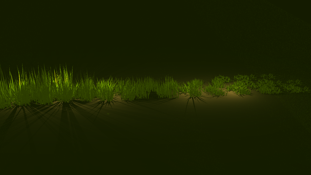
grass_desert.json	46.1
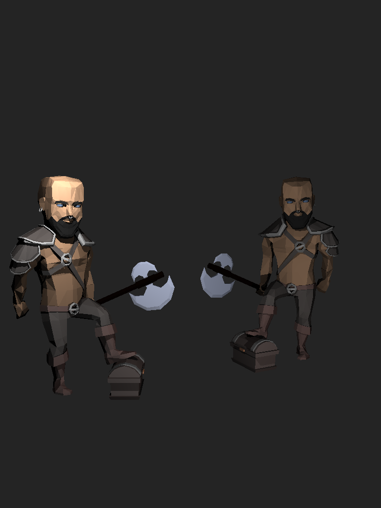
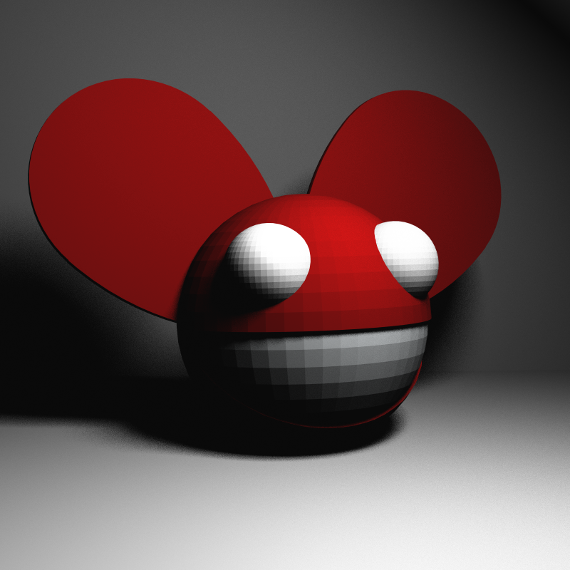
two_berserkers.json	0.5

Stratified Random Sampling and Area Light

Implementing stratified random sampling was quite straight forward. I used the given random sequence generator to generate random values, picked a random position for each sample in its tile, and traced normally for each sample. I also shuffled the sample indices for each pixel and applied Gaussian filtering to calculate the resulting color value. I didn’t encounter any errors during this process, but I didn’t find a noticable difference for the given scenes, perhaps because the scenes didn’t have much aliasing in the first place.

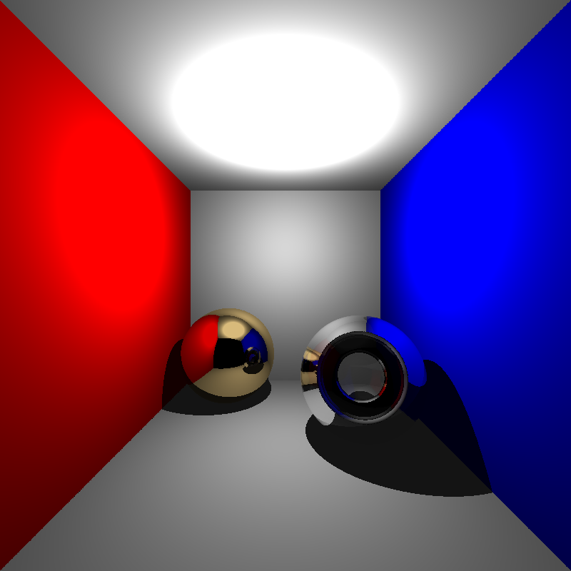
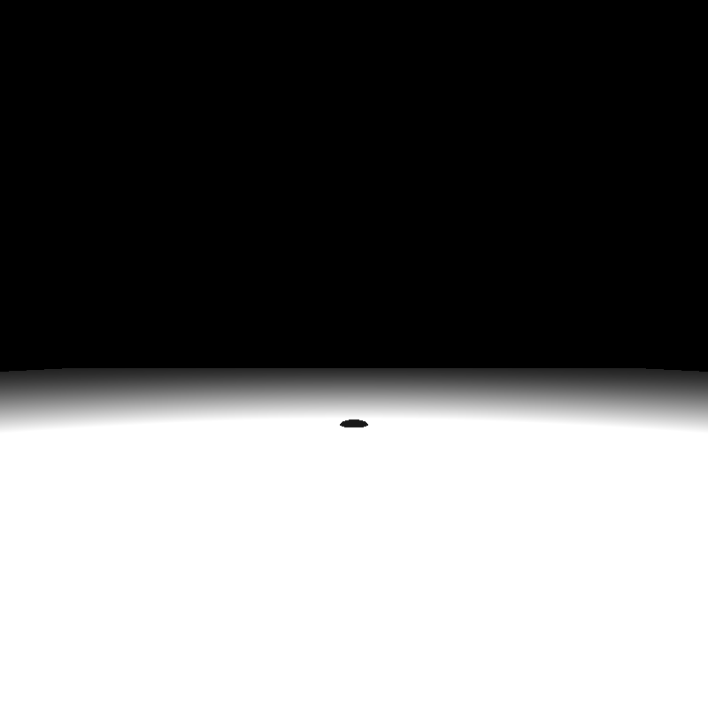
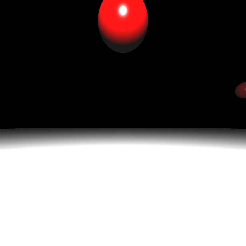
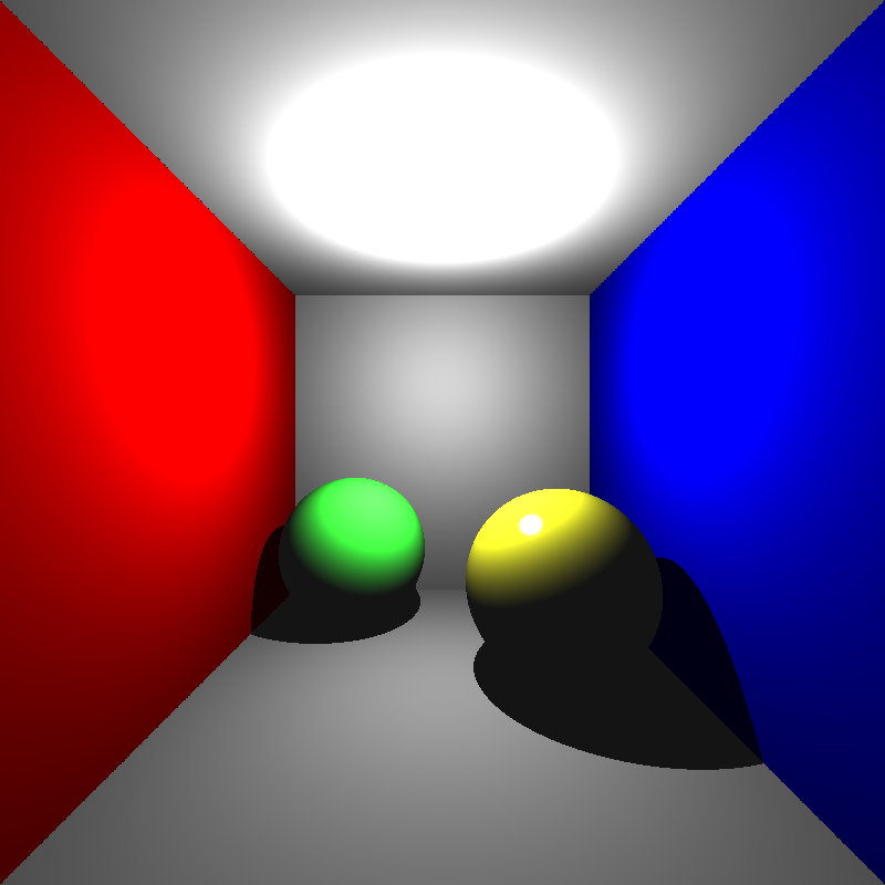
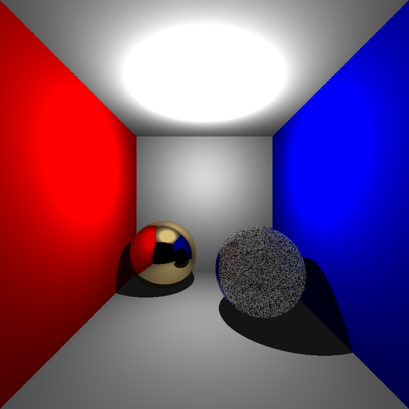
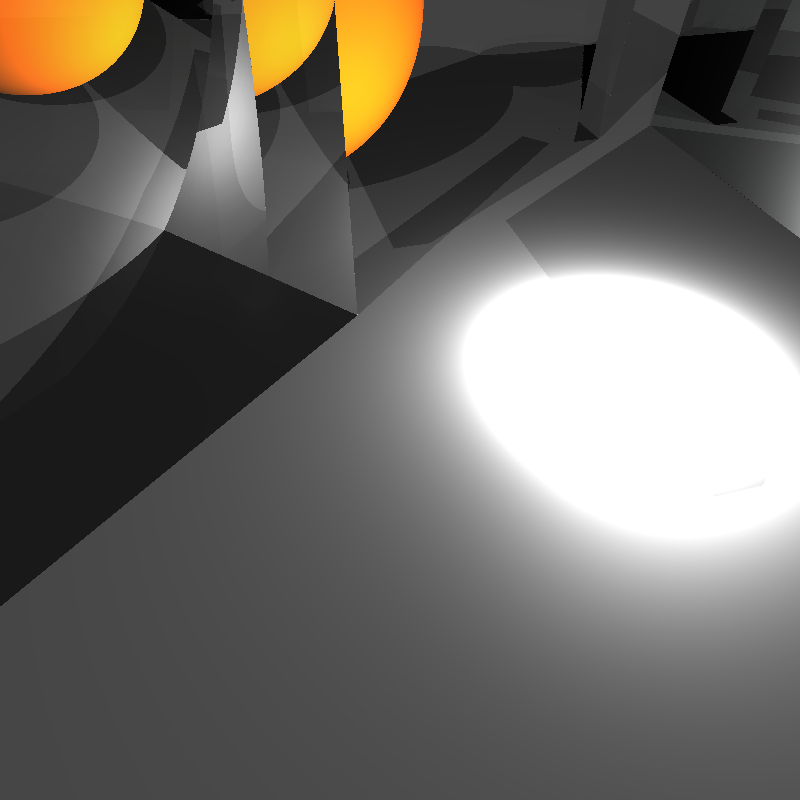
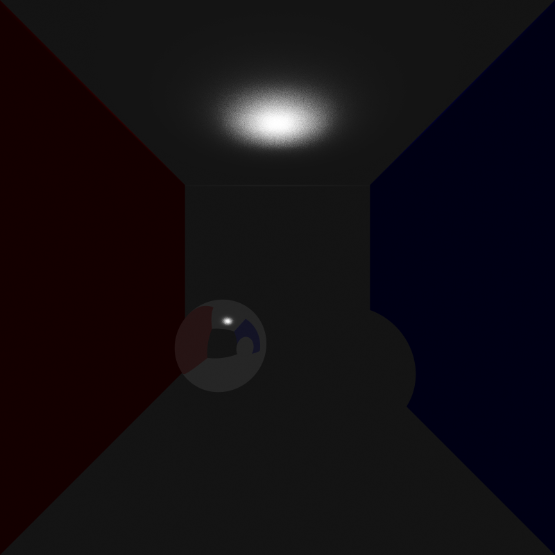
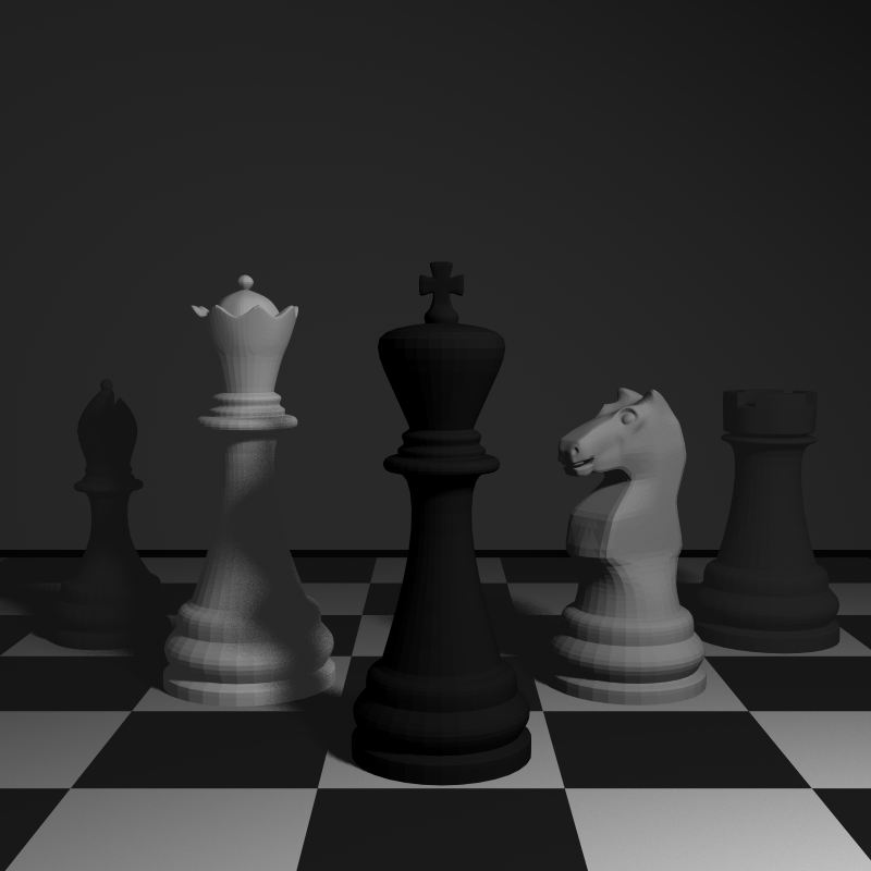
After that, I implemented area lights. I thought implementing area lights would be a simple process as well, but my initial results were quite odd. Below was my first rendering of cornellbox_area.json and chessboard_arealight.json after implementing area lights:

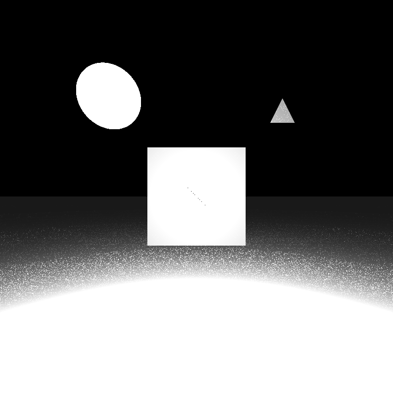
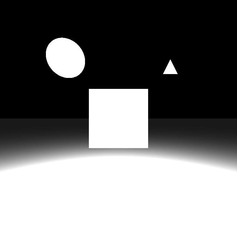
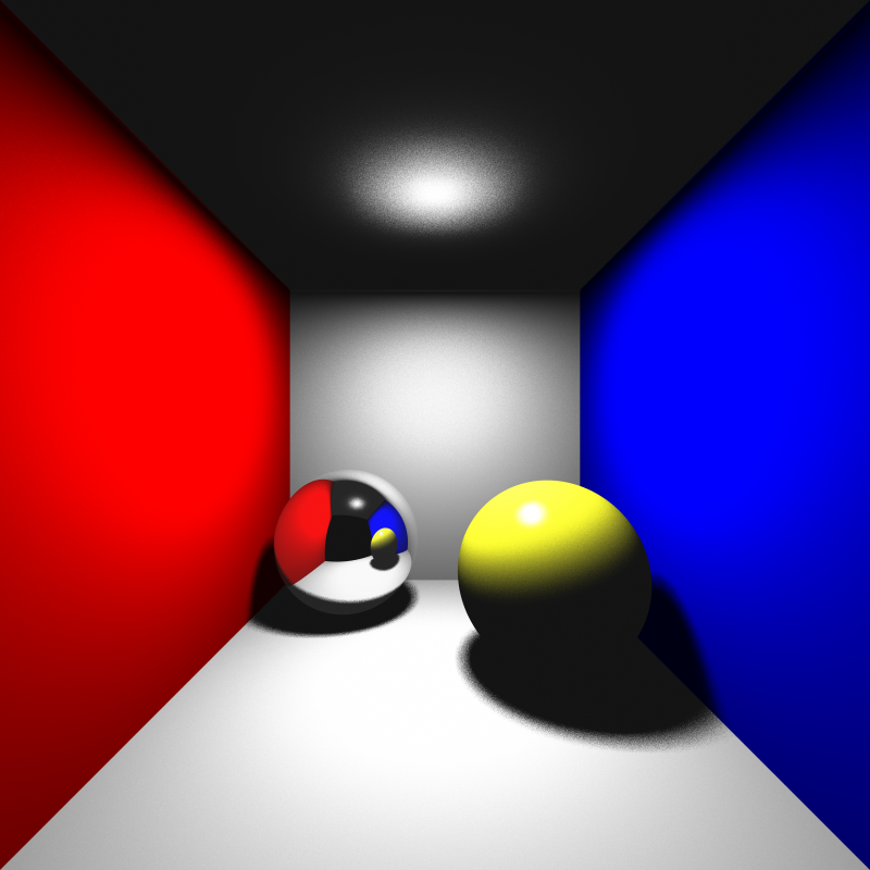
I thought the reason for this might be that I implemented the area lights as one directional. But even after modifying it to be two directional, the rendered images were still really dark. Then I checked if I was calculating the random positions correctly. After checking, I noticed I was adding the random values, which were between 0 and 1, without normalizing them so some of the random points I calculated on the area light were actually outside its area, but this shouldn’t have made the scene so dark. Sure enough, this was not the cause either. After doing a bit of testing, I found out the calculated directions and the shading values were really weird so I tried switching the ordering of the cross product when calculating the arbitrary normal. This worked yet it shouldn’t have, I was already considering the area light as two directional, so changing the ordering should not have made any difference. What was even weirder is that after switching the ordering back again, it still works! I’m still not sure what caused this, but I’ll figure it out another time. Below are the renderings of the two scenes above after my modifications:

Depth of Field

Next in the list was depth of field. After implementing area light, I learned my lesson to normalize the random values when necessary, so I didn’t encounter any problems there. Instead I miscalculated the size of the horizontal and vertical step to find the random aperture sample point. I accidentaly used the image plane width and height instead of pixel width and height which gave the result below when rendering spheres_dof.json:

After fixing this minor issue, I got the correct result:

Motion Blur

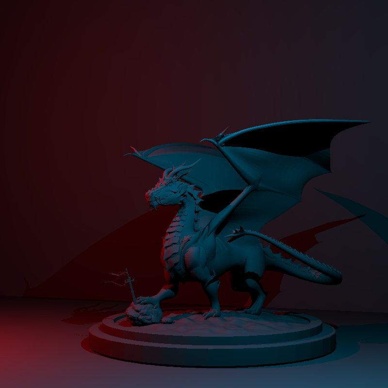
Implementing motion blur was a bit trickier than the previous features as I had to modify my BVH implementation a bit to accomodate objects with motion blur. For those objects, I recalculated their bounding box from both their vertices at t = 0 and t = 1, which gave me the largest extent that included every possible positioning of that object. To calculate intersection with objects that had motion blur, I translated the ray origin in the opposite direction instead of transforming the entire geometry. This implementation gave the result below for dragon_dynamic.json:

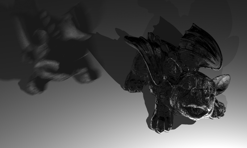
I’m not quite sure why the colors are off, but I didn’t have much time to try to figure out the reason behind it, so I moved on to glossy reflections.

Glossy Reflections

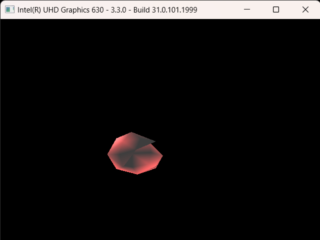
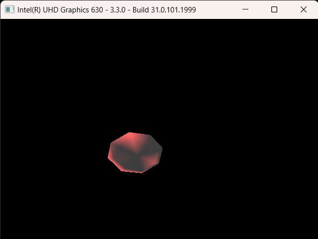
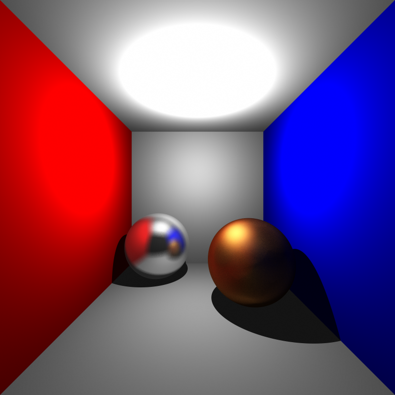
When implementing glossy reflections, I wasn’t quite sure how I should apply the given roughness value, so I decided to simply multiply the offsets by the roughness value itself. Perhaps more interesting results could have been obtained with various roughness functions, but I didn’t want to spend too much time on it, at this point I had an hour or two until the deadline. I calculated the offsets with two random values and obtained the result below for cornellbox_brushed_metal.json:

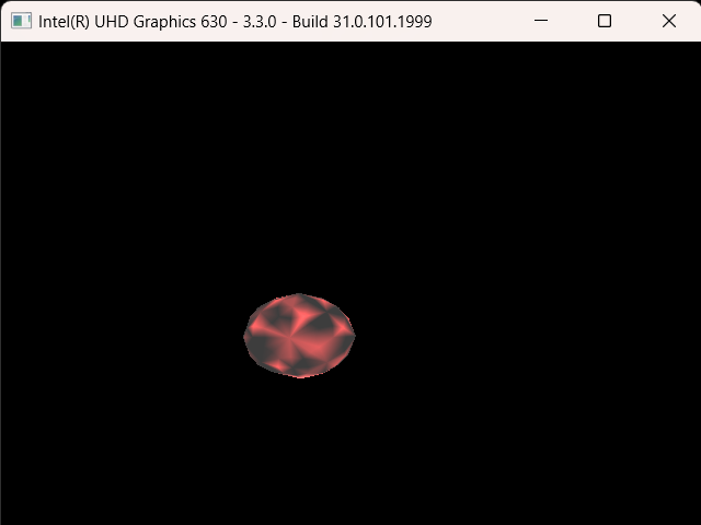
Turns out I hadn’t actually learned my lesson after implementing area lights. I had yet again forgotten to normalize the random values. After normalizing them I got the result below:

Remaining Issues and Render Times

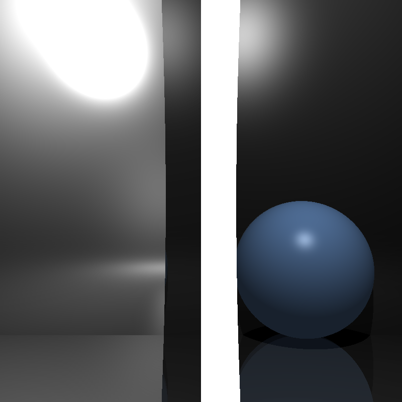
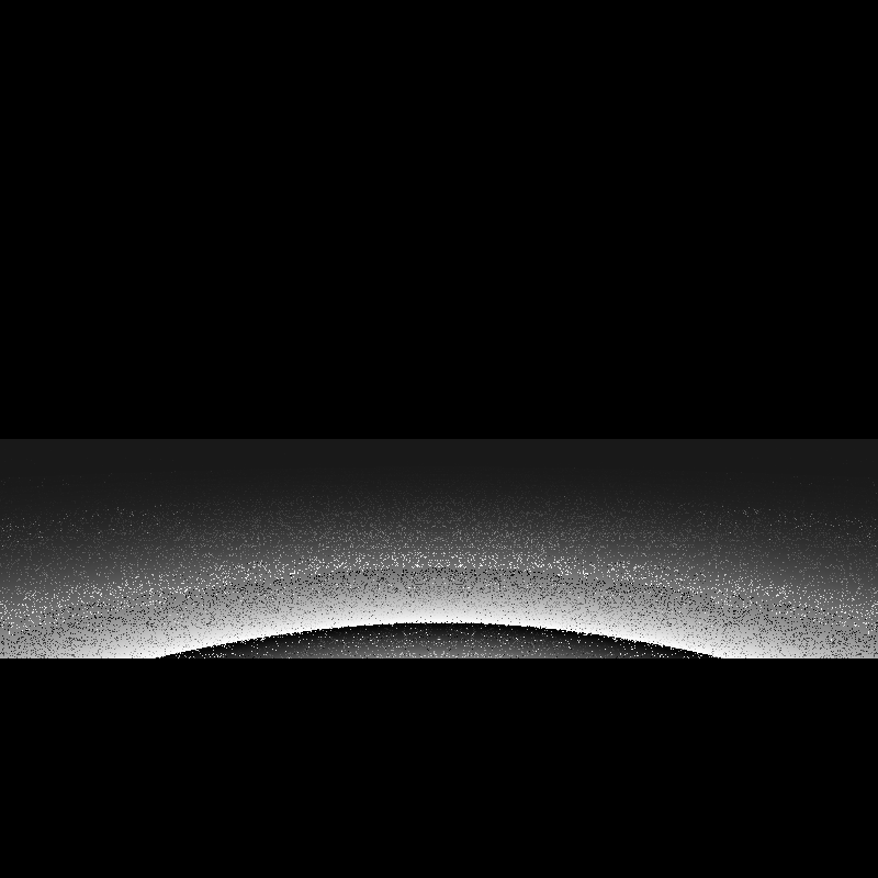
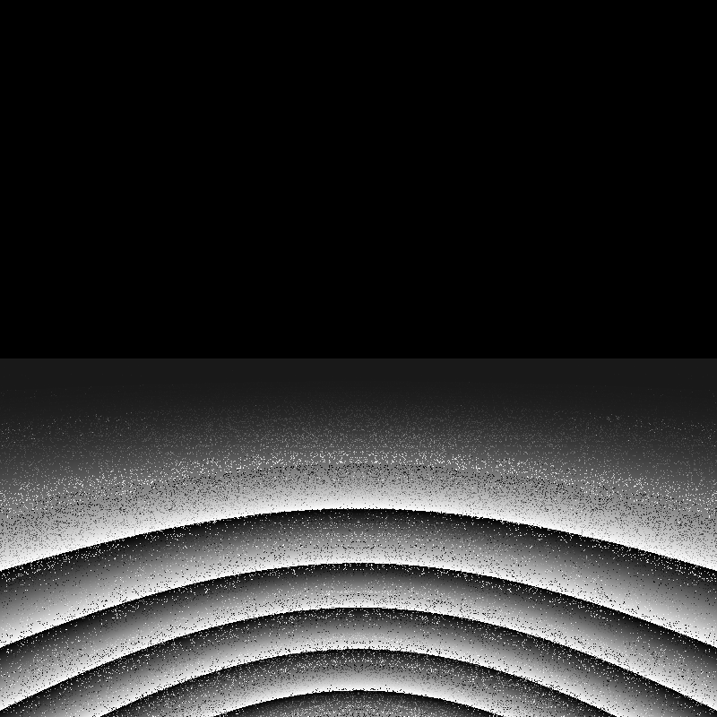
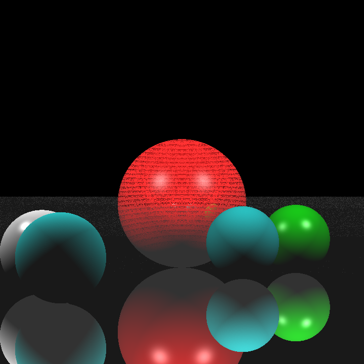
During this blog post I didn’t mention some scenes relevant to the topics I was discussing. That’s because some scenes are rendered completely black for some reason and I have no idea why. While cornellbox_area, cornellbox_brushed_metal, and dragon_dynamic are being rendered just fine, cornellbox_boxes_dynamic and focusing_dragons result in a completely black image. Similarly chessboard_arealight is rendered fine while renderings of chessboard_arealight_dof and chessboard_arealight_dof_glass_queen result in an almost completely dark image with a small patch that is slightly brighter. Unfortunately, I didn’t have time to figure out the reason behind these issues, so hopefully I’ll figure it out while implementing the next homework. Below are some extra scenes and the render times of scenes that produced proper results:

Scene File	Render Time (seconds)
spheres_dof.json	27
cornellbox_area.json	49
cornellbox_brushed_metal.json	190
chessboard_arealight.json	74
metal_glass_plates.json	222
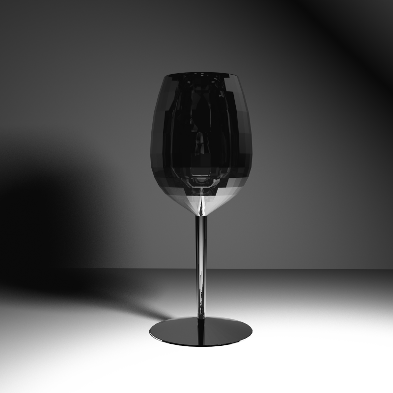
wine_glass	6213
dragon_dynamic.json	27925

For the second homework of my CENG 795: Advanced Ray Tracing course, I tried to expand my previous ray tracer by adding its missing features from the previous homework, adding an acceleration structure (specifically a BVH with median split method), and modifying the parsing and tracing to support mesh instances and transformations. Most of these attempts failed unfortunately. Nevertheless, I will be explaining every step of my implementation and providing some rendered images from my attempts below.

Wrapping the Tracing Process and Re-attempt at Refraction

Before I began implementing the required features of this homework, I believed that I needed to move my tracing functions into a single trace function so that calculating hit detection during BVH traversal would be easier and I could perhaps fix my refraction calculation during this process. I wrapped the tracing process in a single function called trace() that recursively calls for itself when it detects reflection or refraction. The calculations for intersection, color, shadow, and reflection are essentially the same before, but I rewrote my refraction calculation. My refraction calculation now supported multiple reflection and refraction iterations instead of one, and the reflection and refraction weights are clamped in case one of them exceeded 1. The images below are renderings of cornellbox_recursive.json; the top image is rendered by my previous ray tracer, and the bottom image is rendered by my modified ray tracer:

While the dielectric sphere is rendered a lot better (at least parts of the background are visible now) the refractions were still very off. This result was still not quite acceptable, but I did not want to waste too much time on details that were irrelevant to this homework, so I moved on with my implementation.

Applying Transformations

To apply transformations to objects, I decided to store the composite transformations for the object vertices and their inverse transposes for their normals initially. Then I would apply the transformations on each vertex and normal before rendering and calculate intersections through world space. After spending a little time implementing and fixing some minor bugs, this implementation seemed to have worked, at least for simple scenes. But I noticed a problem for spheres that had non-uniform scaling transformations. Below is a rendering of spheres.json when I tried to apply the transformations to the objects:

This result was quite perplexing. The process of calculating the composite transformations and applying them should have been incredibly simple. After going over my implementation, I couldn’t really find any problems either (But there actually was a major problem that I overlooked, much to my dismay. I’ll talk about the problem toward the end of this section). Then I realised something. The radii of the spheres never got transformed. As no multiplication operations could be done on them, the radii would not change and the spheres would still appear as uniform spheres instead of ellipsoids. While I could have multiplied the radius by the common diagonal value for uniform scalings, this would not have worked for non-uniform scalings.

While searching the internet over this issue, I found these posts that had interesting ideas:

https://stackoverflow.com/questions/34220370/apply-matrix-transformation-to-a-sphere

https://math.stackexchange.com/questions/3159618/principal-axes-of-deformed-ellipsoid

Transforming the sphere into an ellipsoid with different principal axes sounded interesting, but it felt like trying to implement something like this would have put too much unnecessary work, so I decided to apply the inverse of the transformation on the ray position and direction for each object and calculate that way.

When I finished implementing it, I got the results below:

The reason for this was incorrect intersection calculation, which was caused by several minor mistakes like using local t values to compare instead of t values for world space and setting the w component of directions (such as ray direction and normal) to 1 instead of 0. Fixing these issues still gave me incorrect results:

Still oddly incorrect results yet I was sure there were no errors in my implementation. After spending a considerable amount of time contemplating over this, I finally found the major problem I mentioned before. The problem was in the order of matrix multiplication. When calculating the composite transformations I put the matrices in incorrect order. The amount of small yet crucial details I managed to overlook is honestly astonishing. I doubt anyone could match me when it comes to that.

With the transformation ordering now fixed, I got the results below:

Somehow the results were still incorrect, but I had had my fill of transformations at this point, so I decided to move onto implementing the BVH.

Implementing BVH, Mesh Instances, and PLY Parsing

I normally intended to explain mesh instances and ply parsing in another section, but I could not implement them in time, so I decided to explain them in this section. This entire section is actually more about my shortcomings as even my BVH implementation seems to be almost useless.

For my BVH implementation I tried to implement a two-level, linear BVH tree with median splitting where each mesh would have its own bottom level BVH tree. For this, I wrote a small bounding box struct that just held the minimum corner, maximum corner, and its center. I then wrote a primitive struct that would represent each object and stored these primitives in the array. Each BVH node would keep track of its primitives by primIndex and primCount. In the BVH tree itself, each node’s left child is in the next index of the parent and the right child is offset by rightOffset. Below is a simplified version of these structs:

struct BBox {
    parser::Vec3f min_corner; // minimum x, y, z of the box
    parser::Vec3f max_corner; // maximum x, y, z of the box
    parser::Vec3f center;

    BBox() {
        min_corner = {0.0, 0.0, 0.0};
        max_corner = {0.0, 0.0, 0.0};
        center  ={0.0, 0.0, 0.0};
    }

    BBox(parser::Vec3f min_vec, parser::Vec3f max_vec, parser::Vec3f center_vec) {
        min_corner = min_vec;
        max_corner = max_vec;
        center = center_vec;
    }
};

struct BVHNode {
    BBox bbox;
    uint32_t firstPrim;     // index in primitives[]
    uint16_t primCount;     // leaf count
    uint16_t rightOffset;   // index offset to right child
    uint8_t  nodeType;      // 0=leaf, 1=interior
};

struct Primitive {
    BBox bbox;
    enum { SPHERE, TRIANGLE, MESH_TRI, MESH_TOP } type;

    parser::Sphere sphere;
    parser::Triangle tri;

    parser::Mesh mesh; // only valid for MESH_TOP
    std::vector<Primitive> meshFaces; // for per-mesh BVH
    std::vector<BVHNode> meshBVH;

    parser::Matrix4f inverse_transform;

    Primitive(parser::Sphere s);

    Primitive(parser::Triangle t);

    Primitive(parser::Mesh m);
};

My structs probably could have been more efficient, but my initial priority was to get a working BVH. I built a BVH recursively and assigned primitives to each split by which side they are on compared to the median of the given bounding box. When I ran my ray tracer on some simple scenes, I got the results below:

Oddly enough, these scenes were now being rendered properly. I couldn’t figure out the reason behind this, but probably there was still something wrong with my intersection calculation.

Unfortunately, I couldn’t implement a parser for PLY files. I tried to use the ply library by Paul Bourke, but I could not get it to work no matter what I did. I also tried to get Google Gemini to produce a parser for me (it was the only model working when Cloudflare was down), but its implementation didn’t work either. For mesh instances, the ones in the example files all referenced PLY meshes as their base meshes, so I couldn’t really get around to implementing that. It felt like it would be pointless if the base meshes did not exist. I didn’t give a table for render time either because the simple scenes that could be rendered take a second at most and I don’t have render times for complex scenes that use PLY files.

In the end, this homework turned out to be less about producing a flawless ray tracer and more about discovering just how many ways I can break one. I was quite impressed by the amount of mistakes I’ve made. In any case, I’ve come to understand the importance of writing modular and maintainable code that can be extended as needed for future use.

For the first homework of my CENG 795: Advanced Ray Tracing course, I implemented a simple ray tracer in C++ that reads scene data from a JSON file and renders images using basic ray tracing methods. My ray tracer performs ambient, diffuse, and specular shading calculations for intersected objects, as well as shadow calculations when the light source is obstructed by another object. Additionally, it performs reflection calculations for mirror, conductor, and dielectric objects, and unfortunately, it incorrectly calculates refraction for dielectric objects. In this post I will explain my implementation process, the errors I came across, and the resulting images with their rendering time. I will also provide some explanations that might be redundant. This is totally for the sake of future visitors who might not be familiar with ray tracing and absolutely not to increase the length of this post.

 

Parsing and Storing the Scene Data

According to the homework specifications, I was required to parse both JSON and PLY files for scene data. I used Niels Lohmann’s JSON library to parse the scene information and stored it using a set of custom structs. Unfortunately, I wasn’t able to implement PLY parsing in time, so my ray tracer currently only works with JSON files.

All scene-related data is contained within a single Scene struct, which includes several other structs corresponding to each field in the JSON file. While the homework document already explains each field, I’ll briefly summarize them here for completeness.

Below is the Scene struct and a brief description of each field:

struct Scene
    {
        //Data
        Vec3i background_color;
        float shadow_ray_epsilon;
        float intersection_test_epsilon;
        int max_recursion_depth;
        std::vector<Camera> cameras;
        Vec3f ambient_light;
        std::vector<PointLight> point_lights;
        std::vector<Material> materials;
        std::vector<Vec3f> vertex_data;
        std::vector<Mesh> meshes;
        std::vector<Triangle> triangles;
        std::vector<Sphere> spheres;
        std::vector<Plane> planes;
        //Functions
        void loadFromJSON(std::string filepath);
    };

• background_color: A vector of integers containing the RGB value of the scene background.
• shadow_ray_epsilon:  A small float value used to offset the intersection points in order to prevent self-intersection.
• intersection_test_epsilon: A small float value that was unspecified in the homework documentation. I initially assumed it was supposed to be used to offset the intersection points while calculating reflections. This has caused quite a bit of headache for me while implementing reflection calculation.
• max_recursion_depth: The maximum amount of times a ray’s bounce will be calculated when reflected.
• cameras: An array of Camera objects, each containing information about the camera vectors and the image plane.
• ambient_light: A vector of floats defining how much light an object receives even in shadow.
• point_lights: An array of PointLight objects, each containing a vector of floats for position and a vector of floats for intensity.
• materials: An array of Material objects, each containing the type of material and the necessary values for shading.
• vertex_data: An array of float vectors, each containing the position of the vertex in the given index.
• meshes: An array of mesh objects, each containing the shading type, the index of the material, and an array of Face objects.
• triangles: An array of Triangle objects, each containing the indices of its vertices, the index of its material, and a float vector representing its normal.
• spheres: An array of Sphere objects, each containing the index of its material, the index of its center vertex, and its radius.
• planes: An array of Plane objects, each containing the index of its material, the index of its point vertex, and a float vector representing its normal.
• loadFromJSON: The function to parse and store the scene data.

Ray Calculation and Object Intersection

To give a bare bones explanation, ray tracing works by tracing a ray for each pixel of an image, checking for any objects intersected along that ray, and calculating the corresponding color based on the material and lighting. My ray tracer is just as bare bones as this explanation, it simply calculates a ray direction for each pixel, checks if any object is intersected, and computes the shading of the object at that point. Despite these simple steps, I made a lot of mistakes in my initial implementation. I’ll first show the results of some minor ones. The images below are all rendered from simple.json:

The image above is the correct rendering of simple.json. When I finally obtained the image above I thought that the base of my ray tracer was now complete. However, when I ran the ray tracer on other sample scenes, I got completely black images. This scene was the only one that was being rendered correctly. Debugging this problem took quite a bit of time.

My first thought was to check if there was something wrong with my intersection functions as no intersection occured at any pixel. I went over my implementations several times, I rewrote the triangle intersection function with matrix structs to make it more readable, I tested them with my own sample values. There was no issue with them.

My second thought was to check if there was something wrong with my calculations for the camera vectors and the image plane. I went over my gaze calculations for cameras with “lookAt” types, checked the corner calculations for the first pixel, yet nothing seemed to be wrong. Since the calculations for the image plane were correct the ray directions should have been correct by extension, or so I thought.

When I checked the ray directions individually while rendering, they turned out to be way off in some scenes. At this point I finally realised the issue: after calculating the pixel position I never subtracted the camera position from it, which gave me a position vector of the pixel instead of the ray direction vector. Since the camera of the simple.json scene was located at (0, 0, 0), the image was rendered correctly, while all the other scenes-which had cameras at different positions-appeared completely black. Fixing this mistake gave me the results below:

Reflection and Refraction Calculations

Next came the task of calculating the reflections and refractions for mirrors, conductors, and dielectrics. I initially just focused on implementing reflections for mirrors to make sure that I got the reflections working correctly first. The image below is rendered from spheres_mirror.json after I finished my initial mirror implementation:

The result was a little off putting. The reflections of the center sphere even looked a little like a creepy, smiling clown. I believe the main reason for this was because I calculated the reflection rays incorrecty, but I wasn’t too sure as my initial implementation was quite messy. So I decided to redo the mirror implementation from scratch in a clearer way. My second mirror implementation gave the result below:

The result was a lot better than the first one, but there were still some noisy pixels scattered in certain areas. Tracking down the cause of this issue took a very long time, I almost decided to just move on and leave it as it was. I went over everything several times, but I couldn’t find anything wrong with my implementation. I redid the mirror implementation, but it still gave me the same result.
Eventually, I decided to tinker with the values inside the scene file. I tried changing almost every value inside the scene file without success until I finally decided to change the epsilon value. It turned out that the intersection_test_epsilon value-which was the value I used to offset the intersection point-was far too small and still caused self-intersection at certain points. When I used shadow_ray_epsilon instead, I got the result below:

At last, my mirror implementation seemed to be working correctly. After that, implementing Fresnel reflections for dielectrics and conductors didn’t take much time at all.
Now it was time for the final hurdle: calculating refractions. At this point I had very little time left so I decided to just implement a single refraction ray that did not bounce after leaving the object, yet even that proved challenging. Once again, the issue was noisy values at certain points but this time I could not come up with a solution. No matter how I changed the offset values or redid the refraction implementation, the result remained the same. Below is the rendering of cornellbox_recursive.json which contains a single conductor sphere to the left and a single dielectric sphere to the right:

Finally, here are the rendering times for various scenes:

Scene	Render Time
simple.json	1 second
spheres.json	1.35 second
spheres_with_plane.json	1 second
spheres_mirror.json	1.36 second
two_spheres.json	0.2 second
cornellbox.json	3.9 seconds
cornellbox_recursive.json	4.7 seconds
bunny.json	312 seconds
chinese_dragon	>12hrs

Despite a few issues along the way, I learned a lot through this assignment. The mistakes I made were simple but taught me valuable lessons about the fundamentals of ray tracing. I’m excited to keep improving my renderer and explore more advanced techniques in the future.

I have implemented procedural city generation on OpenGL and in this blog post, I will explain my implementation process and discuss my results.

My initial plan was to implement the following features:

• Procedural grid rendering using Wang Tiles and noise sampling.
• Building generation using L system grammars and level-of-detail rendering.
• Greenery generation using L system grammars and noise sampling.

In the sections below, I will explain my implementation process for each feature in detail.

Grid Generation

The purpose of generating a grid was to determine the contents of each tile in a manner that would look natural. To achieve this, my plan was to sample from a noise function to determine a few initial tiles, and then generate the rest of the grid by using Wang tiles with appropriate constraints or, if that produced unacceptable results, use Wave Function Collapse to generate the rest of the grid seamlessly.

I initially planned on using Perlin noise through an existing library called ‘stb_perlin.h’. However, its perlin_noise3() function only generated values with very small absolute values (below 0.1 in most cases) for some reason, so I decided to implement the function myself. My first attempt was to utilize the function I used for my third homework in this course. For some reason, it produced a checker-like pattern. The video below shows a 10 by 10 grid that was generated by sampling from my Perlin noise function. To visualize the contents initially, I simply rendered some pictures for each main tile type (grasses for greenery, a straight road for the roads, and a parking lot for the buildings)

While looking for some resources on the technical details of Perlin noise, I came across this video. I decided to reimplement using this video as a guide, and my new function provided much better results:

For this implementation, I used 2D Perlin noise with the following gradient vectors:

const glm::vec2 gradients[8] = {
    glm::vec2(1, 0),
    glm::vec2(-1, 0),
    glm::vec2(0, 1),
    glm::vec2(0, -1),
    glm::vec2(1, 1),
    glm::vec2(-1, 1),
    glm::vec2(1, -1),
    glm::vec2(-1, -1)
};

The interpolation function for this implementation is different from the one on the course slides. Instead of using -6|x|⁵+15|x|⁴-10|x|³+1, it uses 6x⁵-15x⁴+10x³. Other than that, the implementation is mostly similar to the one on our course slides:

int hash(int x, int y) {
    return (((x % 256) + y) % 256) % 8;
}


float fade(float t) {
    return t * t * t * (t * (t * 6 - 15) + 10);
}


float lerp(float a, float b, float t) {
    return a + t * (b - a);
}


float dotGridGradient(int ix, int iy, float x, float y) {
    glm::vec2 gradient = gradients[hash(ix, iy)];
    float dx = x - (float)ix;
    float dy = y - (float)iy;
    return (dx * gradient.x + dy * gradient.y);
}


float perlin(float x, float y) {
    // Determine grid cell coordinates
    int x0 = (int)floor(x);
    int x1 = x0 + 1;
    int y0 = (int)floor(y);
    int y1 = y0 + 1;

    // Determine interpolation weights
    float sx = fade(x - (float)x0);
    float sy = fade(y - (float)y0);

    // Interpolate between grid point gradients
    float n0, n1, ix0, ix1, value;

    n0 = dotGridGradient(x0, y0, x, y);
    n1 = dotGridGradient(x1, y0, x, y);
    ix0 = lerp(n0, n1, sx);

    n0 = dotGridGradient(x0, y1, x, y);
    n1 = dotGridGradient(x1, y1, x, y);
    ix1 = lerp(n0, n1, sx);

    value = lerp(ix0, ix1, sy);

    //return (value + 1) / 2;
    return abs(value);
}

To map the values between 0 and 1 I tried both (n(x,y)+1)/2 and |n(x,y)|. From the tests I’ve done, the second option seemed to yield better results, but this mostly depends on how one maps the tile values to the noise values.

Once I increased the grid size and changed the mapping a bit, I got the following pattern:

The black tiles represent roads, the green tiles represent the greenery, and the greyish tiles that are clumped together represent the building tiles. This produced quite a nice pattern in my opinion. So I increased the size to 100 by 100 and tweaked the mapping just a bit more to produce this pattern:

This pattern looks quite nice in my opinion. The building blocks are grouped together, which should lead to more buildings being generated near each other with greenery tiles between building clusters. I should mention that I used the gradient vectors without random indexing or creating random gradient vectors, so the Perlin noise map is constant. This is fine though, as my plan is to just sample some initial tiles and then start generating from those tiles according to their constraints, leading to varying but consistent patterns. At least, that was my plan.

Once that was done, I tried to add some constraints and generate the tiles according to them. Below are two 25 by 25 grids where the first one was created with 5 samples and the second one was created with 25 samples:

While more samples lead to more variance, the overall pattern looked quite randomized. The reason behind this is my constraints being inadequate. I tried to improve the pattern by adding more tile types and different constraints further on but I couldn’t achieve a good looking pattern.

Tree Generation

To generate trees, I utilized an L system grammar. I was initially also going to sample from a noise function to determine the positions of trees within a tile, but since the tiles were already quite small and the buildings were going to be scaled according to the tiles, I decided to render one tree per greenery tile, and determine the type of tree at that tile by sampling from the mapped Perlin noise values.

The L system I used for the trees works as follows:

Forward (‘F’):

• Calculate the next position by moving forward.
• Add a cylinder segment.
• Update the current position.

Rotate Right (‘+’):

• Rotate by 25 degrees around the Z-axis in a positive direction.

Rotate Left (‘-‘):

• Rotate by 25 degrees around the Z-axis in a negative direction.

Push State (‘[‘):

• Push the current transformation matrix onto the stack.
• Push the current position onto the stack.
• Push the current thickness (as a scale matrix) onto the stack.

Pop State (‘]’):

• Pop the thickness from the stack and update thickness.
• Pop the current position from the stack and update current position.
• Pop the current transformation matrix from the stack and update the current matrix.

Below is the code for this system:

void parseLSystem(const std::string& lSystemString, std::vector<glm::vec3>& vertices, const glm::vec3& startPosition) {
    std::stack<glm::mat4> stack;
    glm::mat4 currentMatrix = glm::translate(glm::mat4(1.0f), startPosition);
    glm::vec3 currentPosition = startPosition;
    glm::vec3 forwardVector(0.0f, 0.5f, 0.0f); // Determines the length over a direction

    float initialThickness = 0.09f;
    float thickness = initialThickness;

    for (char c : lSystemString) {
        if (c == 'F') {
            glm::vec3 nextPosition = currentPosition + glm::vec3(currentMatrix * glm::vec4(forwardVector, 0.0f));
            addCylinderSegment(vertices, currentPosition, nextPosition, thickness);
            currentPosition = nextPosition;
        }
        else if (c == '+') {
            currentMatrix = glm::rotate(currentMatrix, glm::radians(25.0f), glm::vec3(0.0f, 0.0f, 1.0f));
        }
        else if (c == '-') {
            currentMatrix = glm::rotate(currentMatrix, glm::radians(-25.0f), glm::vec3(0.0f, 0.0f, 1.0f));
        }
        else if (c == '[') {
            stack.push(currentMatrix);
            stack.push(glm::translate(glm::mat4(1.0f), currentPosition));
            stack.push(glm::scale(glm::mat4(1.0f), glm::vec3(thickness)));
        }
        else if (c == ']') {
            thickness = glm::scale(stack.top(), glm::vec3(1.0f, 1.0f, 1.0f))[0][0];
            stack.pop();
            currentPosition = glm::vec3(stack.top()[3]);
            stack.pop();
            currentMatrix = stack.top();
            stack.pop();
        }
        thickness *= 0.8f; // Reduce the thickness for the next segment
    }
}

By using this system, I generated 6 different tree structures with different strings. Below are the outputs of each string.

Basic branching tree (“F[+F]F[-F]F”):

Dense branching tree (“F[+F[+F]F[-F]]F[-F[+F][-F]F]”):

Somewhat symmetrical tree (“F[+F[+F]F[-F]]F[-F[+F]F]F[+F]F[-F]”):

Wide spread tree: (“F[+F[+F[+F]F[-F]]F[-F[+F]F[-F]]]F[-F[+F]F[-F[+F]F[-F]]]F[+F]F[-F]”):

High complexity tree (“F[+F[+F[+F]F[-F]]F[-F[+F]F[-F]]]F[-F[+F[+F]F[-F]]F[-F[+F]F[-F]]]F[+F[+F[+F]F[-F]]F[-F[+F]F[-F]]]F[-F]”):

Bifurcating tree (“F[+F[+F]F[-F]]F[-F[+F]F[-F[+F]F[-F]]]F[+F[+F]F[-F]]”):

And below is trees being generated on a 25 by 25 grid:

I was going to implement a function to generate several random tree strings according to the L system rules, but I didn’t have enough time to implement it (I couldn’t even render some leaves for the trees).

Building Generation

To generate the buildings, I again used L system grammars. The building grammar is quite simple:

Wall (‘F’):

• Add a wall segment from current position to next position.
• Rotate by -90 degrees for the next segment.

Window (‘W’):

• Similar to ‘F’, but adds a window segment instead of a wall.

Door (‘D’):

• Similar to ‘F’, but adds a door segment instead of a wall.

Roof (‘R’):

• Add a roof from the current position.

Move Up (‘+’):

• Move upwards by height. Basically creates a new floor.

And here’s the code for the system:

void parseBuildingLSystem(const std::string& lSystemString, std::vector<glm::vec3>& vertices, const glm::vec3& startPosition) {
    std::stack<glm::mat4> stack;
    glm::mat4 currentMatrix = glm::translate(glm::mat4(1.0f), startPosition);
    glm::vec3 currentPosition = startPosition;
    glm::vec3 forwardVector(1.0f, 0.0f, 0.0f); // Forward vector for building segments

    for (char c : lSystemString) {
        if (c == 'F') {
            glm::vec3 nextPosition = currentPosition + glm::vec3(currentMatrix * glm::vec4(forwardVector, 0.0f));
            addBuildingSegment(vertices, currentPosition, nextPosition, WALL);
            currentPosition = nextPosition;
            currentMatrix = glm::rotate(currentMatrix, glm::radians(-90.0f), glm::vec3(0.0f, 1.0f, 0.0f));
        }
        else if (c == 'W') {
            glm::vec3 nextPosition = currentPosition + glm::vec3(currentMatrix * glm::vec4(forwardVector, 0.0f));
            addBuildingSegment(vertices, currentPosition, nextPosition, WINDOW);
            currentPosition = nextPosition;
            currentMatrix = glm::rotate(currentMatrix, glm::radians(-90.0f), glm::vec3(0.0f, 1.0f, 0.0f));
        }
        else if (c == 'D') {
            glm::vec3 nextPosition = currentPosition + glm::vec3(currentMatrix * glm::vec4(forwardVector, 0.0f));
            addBuildingSegment(vertices, currentPosition, nextPosition, DOOR);
            currentPosition = nextPosition;
            currentMatrix = glm::rotate(currentMatrix, glm::radians(-90.0f), glm::vec3(0.0f, 1.0f, 0.0f));
        }
        else if (c == 'R') {
            glm::vec3 nextPosition = currentPosition + glm::vec3(currentMatrix * glm::vec4(forwardVector, 0.0f));
            addBuildingSegment(vertices, currentPosition, nextPosition, ROOF);
        }
        else if (c == '+') {
            currentPosition += glm::vec3(0.0f, 1.0f, 0.0f);
        }
    }
}

This system builds very simple buildings with randomized walls that either have a window or not. The ground floor also has a wall with a door in it. The video below showcases a simple building with a door, two windows, and a wall:

For the buildings, at least, I managed to implement a string generator that randomly generates building strings up to a given height (might be shorter). My implementation randomly generates 5 strings and renders the building from those models. Below is the implementation for it:

std::unordered_map> buildingRules = {
{‘F’, {‘F’, ‘W’}},
{‘W’, {‘F’, ‘W’}},
{‘D’, {‘F’, ‘W’}},
{‘+’, {‘F’, ‘W’, ‘R’}}
};

std::string generateBuildingString(int maxHeight = 3) {
std::string buildingString = “D”;
char lastChar = ‘D’;
int wallCount = 1, currentHeight = 0, constraintCount;

//std::cout << "Entered function\n";
while (currentHeight < maxHeight) {
    //std::cout << "Current string: " << buildingString << "\n";
    constraintCount = buildingRules[lastChar].size();
    char newChar = buildingRules[lastChar][rand() % constraintCount];

    if (newChar == 'F' || newChar == 'W' || newChar == 'D') {
        wallCount++;
    }

    buildingString += newChar;

    if (newChar == 'R') break;

    if (wallCount >= 4) {
        buildingString += '+';
        wallCount = 0;
        currentHeight++;
        lastChar = '+';
    }
    else {
        lastChar = newChar;
    }
}

return buildingString;

}

Unfortunately, I didn’t have much time to write a complex system, I barely had time to create the meshes for the walls and doors and windows.

This basically sums up my implementation. Here’s my final runtime video:

Final Discussions

Unfortunately, my implementation is admittedly very shoddy. I was originally supposed to implement this on Vulkan, but I just couldn’t grasp how Vulkan worked and just wasted most of my time. This is terrible time management on my part, as I’m sure I could have implemented something more concrete with interesting results. I could have tried randomizing the Perlin noise gradients and compare grids generated by Wang tile implementation and pure noise sampling. The trees could be rendered with more complex systems to generate some interesting models. Similarly, buildings could also be rendered in much more varying structure and actual texture instead of plain grey. Moreover, because the buildings had such simple meshes, I couldn’t really simplify the models further for LOD rendering. I even had to design the road textures by hand, yet some of them are rendered in red and I have no idea why. Still, I feel like I’ve learned quite a bit and I’d like to further develop this project in my spare time.

For my third homework as part of the Computer Graphics 2 course, I implemented grass rendering in OpenGL using the geometry shader, Bezier curves, and Perlin noise. In this blog post, I will explain my process of learning and implementing this homework.

Learning More About OpenGL

Before I started implementing this homework, I thought that it might be better if I first had a better grasp on how geometry shaders worked so I took a look at various tutorials on geometry shaders and found some interesting sources. While this section is not really important, I found some sources that I thought were really cool and I just wanted to share them somehow.

While looking through some posts on Reddit, I found a comment under this post suggesting a webpage called The Book of Shaders by  Patricio Gonzalez Vivo & Jen Lowe. It is an interactive website that explains how shaders work in detail, showcases some shaders and their results, and even allows you to rewrite those shaders and display your results in real-time. Below is a little sample shader in the “Uniforms” section that displays a flashing animation:

I also found a blog post called Bezier Curves and Picasso by Jeremy Kun where he explains the process in which he draws Pablo Picasso’s drawing called “Dog” using only Bezier curves. It also has an interactive demo that allows you to edit the control points of each curve, leading to some interesting results:

I understand that the sources I talked about above aren’t really related to the homework. I’ll start explaining my implementation process in the section below.

Grass Rendering Implementation

To implement the grasses, I decided to first randomly generate 1000 grasses with random x and z values with 3 control points, then sample the wind value from a temporary function that oscillates with time, and set the control point values from the geometry shader. I first rendered a bunch of simple green-colored line strips:

I though this was a decent starting point. Even with three control points the grasses looked decent enough. But I only implemented this as a starting point, I’m aware that these are not Bezier curves. I used the function below to generate some oscillating values with time:

float getWindVelocity(float x, float y, float time) {
    return 0.1 * cos(0.1 * x + time*2.0) * sin(0.1 * y + time*2.0);
}

I made use of ChatGPT to generate this function since this was supposed to be just a placeholder for the actual Perlin noise implementation (or so I thought at the time).

After this, I decided to implement the wind speed increase/decrease functionality, which was quite simple. I simply scaled the time variable with a variable that changed with input in the sampling function. Later on, I decided to scale the entire output instead, as it provided smoother swaying motions. In the demonstration below, I utilized the former version:

At this point, I needed to test my implementations with more grass blades that were spread over a larger area, but not all of the grasses were visible. So before I proceeded further with the main implementation, I added camera movements and rotations. The movement part was rather simple, to go forward or backward, simply updated the position by multiplying the Front vector with the speed value I set and added it to the position. To go left or right, I calculated the left and right vectors by taking the cross products of the Up and Front vectors.
The rotation part was a bit trickier. I was initially planning on using quaternions as was showcased in one of our lectures, but I couldn’t get a good grasp on the mechanism and I didn’t have much time, so I went for a simpler solution. I simply calculated the offset from the previous position, incremented the yaw and pitch values with the offsets (making sure that the pitch degree didn’t go over 89 degrees or below -89 degrees), and updated the Front and Up vectors with these values. Below is the implementation:

void mouse_callback(GLFWwindow* window, double xpos, double ypos) {
    if (firstMouse) {
        lastX = xpos;
        lastY = ypos;
        firstMouse = false;
    }

    float xoffset = xpos - lastX;
    float yoffset = lastY - ypos; // Reversed since y-coordinates range from bottom to top
    lastX = xpos;
    lastY = ypos;

    xoffset *= sensitivity;
    yoffset *= sensitivity;

    yaw += xoffset;
    pitch += yoffset;

    // Constrain the pitch
    if (pitch > 89.0f)
        pitch = 89.0f;
    if (pitch < -89.0f)
        pitch = -89.0f;

    glm::vec3 front;
    front.x = cos(glm::radians(yaw)) * cos(glm::radians(pitch));
    front.y = sin(glm::radians(pitch));
    front.z = sin(glm::radians(yaw)) * cos(glm::radians(pitch));
    cameraFront = glm::normalize(front);
}

And here is how it looks:

I was first going to implement the rotation by clicking and dragging on the screen so that the user could resize the window, or make it fullscreen. But unfortunately, I couldn’t really figure it out and I didn’t have much time left, so I had to move on. If resizing is absolutely necessary, the glfwSetInputMode at line 463 could be set to GLFW_CURSOR_NORMAL instead of GLFW_CURSOR_DISABLED. This would prevent the camera from being able to rotate completely because when the mouse reenters the window, the camera gaze starts from the initial position (I’m not sure why). By making the window fullscreen, you can rotate and move around enough to see the entire field.

Now I needed to render the blades as actual Bezier curves. I implemented the Bezier curves by first assigning four equally spaced control points to each grass blade starting from the ground coordinate to the assigned height value. Then, I interpolated 10 vertices between the starting point and the ending point using the functions in the course slides. When I rendered the grasses using triangle strips, I increased the amount to 21 segments. Below is how it looks:

I then rendered the grasses using triangle strips. This part was rather simple as well, I just rendered each segment using 2 vertices that went narrower as it grew higher. Since the deadline is technically not over yet and this is potentially an important part of the homework, I won’t post the implementation itself but here’s how it looks:

Now it was time to implement the keyboard functionalities requested as part of the homework. For changing colors, I made it so that the colors of the grasses rotated between three constant RGB values (green, yellow, white). Because not much was specified for this part, I didn’t waste too much time with it. I also added a ground mesh for a bit more aesthetic, but it didn’t really help much:

I decided to change the heights of the grasses between five values where each time the height is increased, it is scaled by 1.5 and vice versa. In terms of implementation, not much was needed since most of the processing was done on the geometry shaders. I just needed to change the stored grass blade data and reupload it to the VBO. I also decided to add some variance to the starting heights of the grasses to give it a more natural look. Here’s how it looks:

Finally, it was time to implement the Perlin noise functionality I had been procrastinating. Implementing the noise function itself wouldn’t be much of a problem, but I didn’t really know how I should sample from it as time went on. I first implemented the Perlin noise inside the geometry shader using the definitions given in the course slides yet again. While I first planned on implementing it using 2D coordinates, the slide specified that the 3D positions should be used to sample from the noise, so I simply went along with it. In hindsight, it was probably for grass field implementations that were done on a non-level surface (unlike mine), so perhaps my implementation would have looked a bit better if I used 2D coordinates but I’m not really sure. The demonstration below shows the grasses sampling from the first version of my Perlin noise implementation where I tried to add some dependency on time with a simple sin function, wind *= sin(time * windMult):

This result was quite unacceptable, but I didn’t really get a sense of how I could fix this. I realized the blades would bend one way while swaying the other, so I scaled the sampling down a bit at the lower parts of the blade. While this did fix the bending issue, the overall swaying animation looked way too stiff even if I capped the amount of swaying at a certain level.
As I was out of both ideas and time, I decided to utilize my so-called ‘temporary’ sampling function again to create a more natural-looking animation. It’s not that I didn’t use my Perlin noise implementation; I did, but instead of the coordinates, I passed the sampled noise values to the oscillating function. The outcome was serviceable, but obviously there is still much that could be done:

I also did some fps calculations on my own computer for the final version (fps was capped at 60 on the ineks):

	FPS (Window mode)	FPS (Fullscreen)
10,000 blades	950-1000	350
20,000 blades	500	200-250
40,000 blades	300	150-170
80,000 blades over larger area	250	90-120

And here’s a guide on the controls of the scene just in case. I have also added the guide in the readme file:

Q: Close the scene.

A/D: Increase/Decrease the wind speed. (0 to 3)

W/S: Increase/Decrease the grass blade length (0 to 4)

E/R: Cycle through the grass colors.

Arrow Keys: Camera movement.

This concludes my grass rendering implementation on OpenGL using Bezier curves, geometry shaders, and Perlin noise. While the base requirements have been met, there are still many features that could be added (skybox, non-level ground distribution) and areas that could be improved further (noise sampling, shading of the grasses). But, I still learned quite a bit from this assignment.

Welcome to my blog page. For my first assignment in the Computer Graphics 2 course, I implemented the Catmull-Clark Subdivision Surface algorithm, and in this post, I will be explaining my process of implementing this algorithm and the errors I encountered along the way.

To understand how the algorithm worked, I first tried to go over the paper “Recursively generated B-spline surfaces on arbitrary topology meshes” by E. Catmull and J. Clark, and the algorithm’s Wikipedia page. I also found a video that gives a simple step-by-step explanation of the algorithm, which helped clear up some parts I didn’t quite understand in the first two sources I mentioned. You can access the video through the following link: https://youtu.be/mfp1Z1mBClc?si=3LienRGDQvvMI0ht

Once I had a clear understanding of the algorithm, I started on my implementation. My initial thought was that it would be better to first write the algorithm itself. Once that was done, I could take care of the rest of the specifications given in the homework document (which was a mistake in hindsight), so I started writing a function on the sample code provided by the assistants.

Throughout writing my implementation, the main problem has always been calculating the vertex normals properly. Once my first implementation was done, I added an octahedron object and tested it. Below is the output:

The reason my output was like this was I believe because I forgot to add the newly calculated faces, but I’m not too certain. It was a minor mistake I had made and I fixed it relatively quickly. The main issues started after I fixed this issue.

Above are the outputs when the subdivision is applied once and then twice, in order. At first glance, I thought that maybe my algorithm was completely wrong, but I realized that the positions of the vertices seemed to be correct. Moreover, it seemed like for every new face I created half of it would not properly render. Since I had separated each new face into two triangles, I was most likely calculating the normal values incorrectly. Unfortunately, no matter what I did I could not fix this issue.

I was calculating the normals by first calculating the vectors going from the new face point to the edges and the corner. For example, let’s say that the new face I was calculating contained a new face point f, two edge points e1 and e2 that neighbored this face point, and a newly calculated vertex p that was between these two edges. I calculated three vectors: one from point f to point e1 (fe1), another from point f to point p (fp), and a third from point f to point e2 (fe2). Next, I computed the cross-products of the vectors fp and fe1, as well as fe2 and fp. Finally, I took the average of these cross-products and added their values to the normals of these vertices.
As one can tell from the results above, there was something wrong with this process. But as I mentioned before, the positions of the new vertices were, at least seemingly, correct, so there had to be something wrong with my normal calculation, at least that is the only possibility that came to my mind. I tried to switch the ordering when doing the cross-products, and the correctly rendered and incorrectly rendered faces seemed to switch. But for some reason when I kept one of the cross-product operations as it was, the entire object was incorrectly rendered.
I tried various other methods from taking the average of all of the normals of faces that were adjacent to a vertex to rewriting the entire function from scratch, but nothing I tried managed to fix this issue. Unfortunately by this point, I was running out of time, and I still had a lot to do so I decided to move on and maybe take a look again once everything else was done.

For the given assignment, I had to prepare a scene with multiple objects that were doing various movements. I decided to keep it simple and decided that I would add four objects, two of which would move perpendicular to each other and cross paths, and the other two would spin around themselves at opposite corners. It initially looked as it did below, with only an octahedron and a tetrahedron moving perpendicularly to each other:

To render multiple objects with their own vertex and fragment shaders, I used the model class my homework partner and I utilized for our final assignment in the Computer Graphics 1 course. I also had to implement a line mode and a wire mode visualization, which were relatively simple to make. The only issue was that there was some aliasing when the visualization was switched to line mode, and changing the glPolygonOffset did not help. As a small workaround, I instead increased the line width very slightly when drawing in line mode. Below is the visualization of line mode with aliasing:

And below is the version with fixed aliasing:

Once that was done, I implemented the functionality to decrease the subdivision level of the objects. Perhaps this might not be the most optimal solution in terms of memory, but I decided that it would be best to simply store the vertex, face, texture, and normal values of each object at each calculated level and simply reuse them when the subdivision level is decreased or re-increased. I understand that this solution might not translate well to a real-life scenario but since the subdivision operation would only be applied a maximum of four times per object, and my subdivision function was very inefficient, I believed that this would be the best solution.
Now, of course, there was a slight issue initially. When I first implemented this, most of the vertices would disappear when the subdivision level was decreased. By this point, I was a bit sleep-deprived so this situation left me a bit perplexed. The video below shows this error:

When I observed this error with a clearer head, I noticed something important: the remaining vertex count when decreasing the subdivision level is actually the amount it was supposed to be at that level, it was just the information of the vertices, faces, and whatnot that was not being updated. Then it dawned on me.

I had forgotten to re-initialize the models after decreasing the levels.

To say this infuriated me would be an understatement as it took an embarrassingly long time to figure this out, which left me with very little time, and I still had to go over my subdivision implementation again. Luckily I at least managed to finish the rest of the requirements. I think.
Below is how it is actually supposed to look. I also added some shading and a new object to the scene:

As I said before, I had decided that my scene would contain 4 objects, yet I’ve only shown 3 so far. The last one is the cube that I had to include in my scene as an obligation of the assignment. But what I had not known was that this cube consisted of quads instead of triangles. Now, this was actually mentioned to us during the briefing of the assignment, I think, but I had forgotten and had failed to properly read the assignment document, which also mentioned that there would be quad topologies (perhaps I’m legally blind).
Realizing this, I quickly started rewriting my parser function so that it could also parse quad objects. I achieved this by dividing each quad into two triangles and writing them to the buffers. I also kept the information of the quads so that I could use them when calculating the subdivision of the cube.
Below is the scene with the cube added:

Finally, I rewrote the subdivision function so that it could also work on quad topology. Unfortunately, my normal calculations were, again, incorrect so the cube was rendered incorrectly yet again.
Below is a video showcasing the final version of my program:

By this point, I barely had any time so I submitted my homework in this state. There were many things I could have improved, or properly implemented, but I mismanaged my time and underestimated the time needed to complete this homework. But still, I believe it is decent enough for homework that was done in three days, at least considering my own capabilities.