6.4. DYNAMIC FORCE ANALYSIS OF MACHINERY
In this section we shall assume that the motion of the machine parts are specified beforehand, e.g. the position velocity and acceleration of each rigid body is known or can be calculated by performing kinematic analysis. We shall also assume that the mass and the moment of inertia of each machine member is known or can be calculated from the given data. There may be external forces of known magnitude and direction or friction forces present. However, we shall assume that there is one external force (such as the input torque) of an unknown magnitude but of a known direction and a point of application. The system is in a state of dynamic equilibrium under the action of these forces. We would like to determine the joint forces, forces acting on the members and the magnitude of the unknown external force.
The above problem is commonly known as kinetostatics or Wittenbauer’s second problem. Such a formulation is valid under steady state conditions and when the mechanism involved is a constrained mechanism. The input speed(s) must be almost constant for these assumptions to be valid or the changes in the velocity and acceleration of the input link is determined by some other means.
Example:
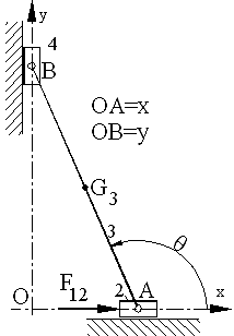
Figure shows a double-slider mechanism. Link 2 is moving with a constant velocity at 2 m/s in positive x-direction. Link 3 is a thin rod of mass m3 = 5 kg and length AB = 500 mm. The masses of links 2 and 4 are negligible. Determine the force F12 acting on link 2 and the joint forces that occur when the mechanism is in the given state of motion and when x = 200 mm. Assume the mechanism is operating on a horizontal plane so that we can neglect the gravitational acceleration. Also neglect friction.
As a first step, kinematic analysis must be performed. Writing the loop equation:
x + a3eiθ13 = iy
Equating the real and imaginary parts:
cosθ = –x/a1
y = a1sinθ
Substituting x = 200 mm we obtain: θ = 113.578° and y = 458.258 mm.
Differentiation of the above equations give us the velocity:
ω13 = \displaystyle \frac {\dot{\text{x}}}{{\text{a}_3}\text{sinθ}} = 4.364 rad/s (CCW)
\displaystyle \dot{\text{y}} = a3ω13cosθ = −872.872 mm/s
The second differentiation yields ( \displaystyle \ddot{\text{x}} = 0):
α13 = \displaystyle \frac {-{\text{ω}_{13}}\dot{\text{x}}\text{cosθ}}{{\text{a}_3}\text{sin}^{2}\text{θ}} = 8.312 rad/s2 (CCW)
\displaystyle \ddot{\text{y}} = −a3ω132sinθ + a3ω13cosθ = −10.390 m/s2
The position, velocity and acceleration of point G3 is:
\displaystyle \vec{\text{r}}_{\text{G3}}=\text{x}+\frac{1}{2}\text{a}_3\text{e}^\text{iθ}
\displaystyle \vec{\text{v}}_{\text{G3}}=\dot{\text{x}}+\frac{1}{2}\text{ia}_3\text{ω}_{13}\text{e}^\text{iθ}
\displaystyle \vec{\text{a}}_{\text{G3}}=\ddot{\text{x}}+\frac{1}{2}\text{a}_3\text{e}^\text{iθ}\left(\text{α}_{13}-\text{ω}_{13}^2\right)
Substituting the known values:
aG3 = 5.194e–iπ/2= 5.194 m/s2 ∠270°
In the second step, we must determine the inertia forces and torques. From Table 1.4 for a thin rod IG3 = \displaystyle \frac{1}{12}ml2. Hence IG3 = 0.10417 kg·m2 and:
F3i = –maG3 = 25.97 N ∠90°
TG3i = –IG3α13 = 865 N·mm (CW)
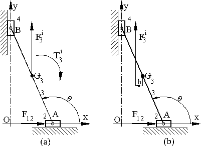
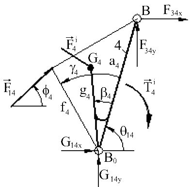
These forces are as shown in the figure below. If a graphical solution is to be performed, inertia force and torque can be replaced by a single resultant (as shown in the figure on right), which is at a distance h from the center of gravity.
h is given by: h = TG3i/F3i = 33.31 mm.
For the force analysis we proceed as if the inertia forces were external forces and apply the methods that were described before for force analysis.
Graphical Method:
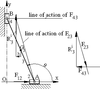
Link 4 is a two force, link 3 and link 2 are three force members.and. For link 3, since R3i is known, we determine the point of concurrency of the three forces and draw the force polygon for the equilibrium equation R3i + F23 + F43 = 0 as shown in the figure. For link 4, G14 = –F34 = F43. For link 2, F32 + F12 + G12 = 0. Since F32 = –F23, the force polygon for the equilibrium equation is that drawn for link 3 with all the arrows reversed. Hence G12 = –R3i and F12 = –F43.
Analytical Method

In the analytical method, since the moment and force equilibrium equations are going to be used separately, one needs not combine the inertia force and torque into a single resultant. The free body diagrams of the moving links are as shown in the above figure.
Since:
F43 = F43 ∠180°
F3i = 25.97 N ∠90°
For link 3 the equilibrium equations are:
F43 – F23x = 0
F3i – F23y = 0
and the moment equilibrium about point A is:
500 F43 sin(180° – 113.578°) + 250 (25.97) sin(90° – 113.578°) – 865 = 0
or
458.258 F43 = 3461.981
F43 = 7.555 N ∠180° F32= –F23 = 27.04 N ∠106.22°
F23x = 7.555 N ∠0° F12 = 7.555 N ∠0°
F23y = 25.97 N ∠270° G12 = 25.97 N ∠270°
F23 = 27.04 N ∠–73.78° G14 = F43
6.4.1. Dynamic Force Analysis of a Four-Bar Mechanism
In order to design links and joints one must determine the worst loading conditions of each link and joint. In order to select the driving motor characteristics, input torque for the whole cycle is required. In such cases analytical methods suitable for numerical computation is utilized. In this part a general dynamic analysis of a four-bar mechanism will be explained and the results will be applied to a particular four-bar for a complete force analysis.

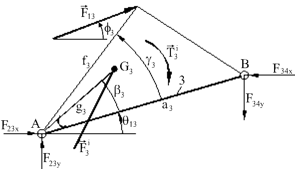
Referring to the figure, the equations for the position, velocity and acceleration analysis of the four-bar mechanism are:
Position Analysis
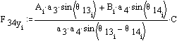
r cosϕ = a1 cosθ12 – a1
r sinϕ = a1 sinθ12
λ = cos-1 \displaystyle \left(\frac {{\text{a}_4}^2+{\text{r}}^2-{\text{a}_3}^2}{2\text{a}_4\text{r}}\right)
μ = cos-1 \displaystyle \left(\frac {{\text{a}_3}^2+{\text{a}_4}^2-{\text{r}}^2}{2\text{a}_3\text{a}_4}\right)
θ14 = ϕ – σλ
θ13 = θ14 – σμ
Note that rcosf and rsinf terms must be solved for r and f simultaneously and the correct quadrant must be ensured. The term s = ±1 depending on whether the mechanism is of open or cross configuration.
Velocity Analysis:
\displaystyle {{\text{ω}}_{{13}}}=\frac{{{{\text{a}}_{2}}}}{{{{\text{a}}_{3}}}}\frac{{\sin \left( {{{\text{θ}}_{{12}}}-{{\text{θ}}_{{14}}}} \right)}}{{\sin \left( {{{\text{θ}}_{{14}}}-{{\text{θ}}_{{13}}}} \right)}}{{\text{ω}}_{{12}}}
\displaystyle {{\text{ω}}_{{14}}}=\frac{{{{\text{a}}_{2}}}}{{{{\text{a}}_{4}}}}\frac{{\sin \left( {{{\text{θ}}_{{12}}}-{{\text{θ}}_{{13}}}} \right)}}{{\sin \left( {{{\text{θ}}_{{14}}}-{{\text{θ}}_{{13}}}} \right)}}{{\text{ω}}_{{12}}}
Acceleration Analysis
\displaystyle {{\text{α}}_{{13}}}=\frac{{{{\text{a}}_{2}}{{\text{α}}_{{12}}}\sin \left( {{{\text{θ}}_{{12}}}-{{\text{θ}}_{{14}}}} \right)+{{\text{a}}_{2}}{{\text{ω}}_{{12}}}^{2}\cos \left( {{{\text{θ}}_{{12}}}-{{\text{θ}}_{{14}}}} \right)+{{\text{a}}_{3}}{{\text{ω}}_{{13}}}^{2}\cos \left( {{{\text{θ}}_{{13}}}-{{\text{θ}}_{{14}}}} \right)-{{\text{a}}_{4}}{{\text{ω}}_{{12}}}^{2}}}{{{{\text{a}}_{3}}\sin \left( {{{\text{θ}}_{{14}}}-{{\text{θ}}_{{13}}}} \right)}}
\displaystyle {{\text{α}}_{{14}}}=\frac{{{{\text{a}}_{2}}{{\text{α}}_{{12}}}\sin \left( {{{\text{θ}}_{{12}}}-{{\text{θ}}_{{13}}}} \right)+{{\text{a}}_{2}}{{\text{ω}}_{{12}}}^{2}\cos \left( {{{\text{θ}}_{{12}}}-{{\text{θ}}_{{13}}}} \right)+{{\text{a}}_{3}}{{\text{ω}}_{{13}}}^{2}-{{\text{a}}_{4}}{{\text{ω}}_{{14}}}^{2}\cos \left( {{{\text{θ}}_{{13}}}-{{\text{θ}}_{{14}}}} \right)}}{{{{\text{a}}_{4}}\sin \left( {{{\text{θ}}_{{14}}}-{{\text{θ}}_{{13}}}} \right)}}
The above equations can be written in different forms.
Acceleration of the centers of gravity
aG2x = −g2ω122cos(θ12 + β2) − g2α12sin(θ12 + β2)
aG2y = −g2ω122sin(θ12 + β2) + g2α12cos(θ12 + β2)
aG3x = −a2ω122cosθ12 − a2α12sinθ12 − g3ω132cos(θ13 + β3) − g3α13sin(θ13 + β3)
aG3y = −a2ω122sinθ12 + a2α12cosθ12 − g3ω132sin(θ13 + β3) + g3α13cos(θ13 + β3)
aG4x = −g4ω142cos(θ14 + β4) − g4α14sin(θ14 + β4)
aG4y = −g4ω142sin(θ14 + β4) + g4α14cos(θ14 + β4)
Using the above equations, one can determine the angular acceleration of the links and the linear accelerations of the centers of gravity for any input condition (input position, velocity and acceleration).
For dynamic force analysis in addition of the inertia forces, we shall assume known external forces F13 and F14 acting on links 3 and 4 and an unknown torque, T12 acting on link 2 as shown in the figure. The system is in dynamic equilibrium under the action of these forces. We would like to determine the input torque and the joint reaction forces.
Note that:
F2i = −m2aG2 , F3i = −m3aG3, F4i = −m4aG4 and T2i = −IG2α12 , T3i = −IG3αG3 , T4i = −IG4α14
The free body diagrams of each moving link can be drawn and the equilibrium equations can be written:
For link 4:
| F34x + G14x + F14cosϕ4 − m4aG4x = 0 | (1) |
| F34y + G14y + F14sinϕ4 − m4aG4y = 0 | (2) |
| F34ya4sin(π/2 − θ14) + F34xa4sin(−θ14) + F14f4sin(ϕ4 − θ14 − γ4) − I4α14 − m4aG4xg4sin(−θ14 − β4) − m4aG4yg4sin(π/2 − θ14 − β4) = 0 | (3) |
For link 3:
| F23x − F34x + F13cosϕ3 − m3aG3x = 0 | (4) |
| F23y − F34y + F13sinϕ3 − m3aG3y = 0 | (5) |
| F34xa3sin(π − θ13) + F34ya3sin(−π/2 − θ13) + F13f4sin(ϕ3 − θ13 − γ3) − I3α13 − m3aG3xg3sin(−θ13 − β3) − m3aG3yg3sin(π/2 − θ13 − β3) = 0 | (6) |
For link 2:
| −F23x + G12x − m2aG2x = 0 | (7) |
| −F23y + G12y − m2aG2y = 0 | (8) |
| F23xa2sin(π − θ12) + F23ya2sin(−π/2 − θ12) + T12 − I2α12 − m2aG2xg2sin(−θ12 − β2) − m2aG2yg2sin(π/2 − θ12 − β2) = 0 | (9) |
Hence, we obtain nine linear equations in nine unknowns (G14x, G14y, F34x, F34y, F23x, F23y, G12x, G12y and T12). If a computer subroutine for the matrix solution is available, these equations can be solved directly for the unknowns. However, it is much simpler to solve equations (3) and (6) simultaneously for F34y and F34x and then solve for each unknown from the remaining equations. The solution is as follows:
A = I4α14 + m4g4[aG4y cos(θ14 + β4) − aG4xsin(θ14 + β4)] − F14f4sin(ϕ4 − θ14 − γ4)
B = I3α13 + m3g3[aG3y cos(θ13 + β3) − aG3xsin(θ13 + β3)] − F13f3sin(ϕ3 − θ13 − γ3)
F34x = [Aa3cosθ13 + Ba4cosθ14]/[a3a4sin(θ13 − θ14)]
F34y= [Aa3sinθ13 + Ba4sinθ14]/[a3a4sin(θ13 − θ14)]
G14x = −F34x + m4aG4x − F14cosϕ4
G14y = −F34y + m4aG4y − F14sinϕ4
F23x = F34x + m3aG3x − F13cosϕ3
F23y = F34y + m3aG3y − F13sinϕ3
G12x = F23x + m2aG2x
G12y = F23y + m2aG2y
T12 = F23ya2cosθ12 − F23xa2sinθ12 + I2α12 + m2g2[aG2ysin(θ12 + β2) − aG2xsin(θ12 + β2)]
One can as well use the principle of superposition and consider forces acting on each link at one time and later add all the force components to find the resultant joint forces. The equations thus found will be similiar to the ones obtained above (written in a different form). This is left as an exercise.
Example:
The four-bar mechanism shown in is used to cut running strip of material. The input link is rotating at a constant speed of 900 rpm CCW. The link dimensions are: |A0A| = 85 mm, |AB| = 235 mm, |B0B| = 550 mm, |BC| = 238 mm, |AC| = 467 mm, |B0C| = 487 mm, ∠BAC3 = 7.6°, ∠BB0C4 = 25.6°. Using AutoCad solid modeller, the mass properties for links 3 and 4 are found as m3 = 2 kg, k3 = 268 mm (radius of gyration), |AG3| = 231 mm, ∠BAG3 = 1° (CW), m4 = 5.1 kg, k4 = 424 mm, |B0G4| = 305 mm, ∠BB0G4 = 7° (CW). For link 2, m2 = 3 kg, k2 = 100 mm and its center of mass is coincident with A0. We are to determine the required input torque and the joint reaction forces. We can neglect friction. A cutting force of 2000 N acts vertically on both links 3 and 4 at point C when the crank angle is 124° < θ12 < 156°. MathCad solution for this example is as follows:
Link dimensions:
![]()
![]()

![]()
![]()
![]()
Constant speed is assumed:

![]()
Increment crank angle for every 2 degrees:
![]()
![]()
![]()
m is crank angle in degrees. Solve for position variables:
![]()
![]()
![]()
![]()
![]()

The angular speed and acceleration of the links are as follows: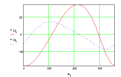

Acceleration of the centers of mass of the links (in mm/s2):
![]()
![]()
![]()
![]()


Mass properties (mass in kg and the radii of gyration, ki, in mm):
![]()
![]()
![]()
![]()
![]()
![]()
![]()
This constant C is to be used to convert mm to m (note that 1kg m/s2 = 1 N). The external forces:
![]()
![]()
![]()
![]()
![]()
![]()
![]()
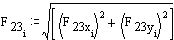
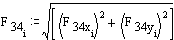
This external force will act vertically on both links 3 and 4 in opposite direction. Determine the joint forces and the input torque (note that the joint forces are in Newtons and the torque is in Newton-meters):


![]()
![]()
![]()
![]()
![]()
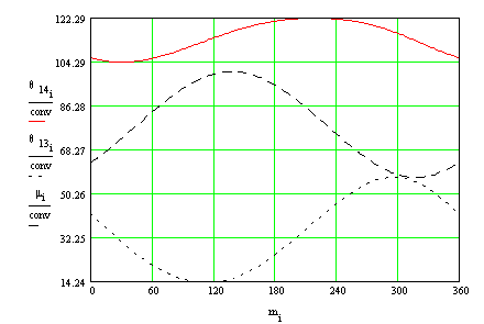
Input torque as a function of crank angle:
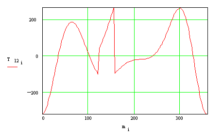
Convert the forces to polar form and plot the forces in a polar plot:
![]()
![]()
![]()
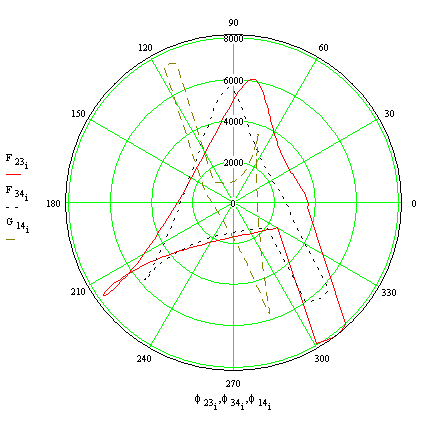
![]()
![]()
![]()
![]()
![]()