6.2.2. Principle of Superposition:
In the previous examples, there was only one known external force acting on one member of the mechanism and the system was brought to static equilibrium by an input or output force (or torque). The magnitude of this force or torque was an unknown. If there are two or more known external forces acting on one link, these forces can be combined into a single resultant and the problem reduces to the case we have already discussed. However, in real machinery there are several external forces acting on different links. For example, if we do not neglect the weight of the members, there will be at least one known external force on each link. In such a case, if we draw the free body diagrams of the links, no simplification will be possible and one has to write three equilibrium equations for each link. The resulting 3(l − 1) linear equations will include 3(l − 1) unknown joint force components and the input force (or torque). Usually simultaneous solution of the equilibrium equations would be required.. Another solution method the principal of superposition. This principal states that the effect of the forces is the sum of the individual effects of the forces considered separately. In other words, if there are two or more external forces present, one can neglect all but one of the forces and determine the joint forces and the unknown reaction force that brings the system into equilibrium for this one external force. If the above procedure is carried out for each of the external forces, at each joint there will be different joint forces corresponding to each external force. The resultant joint force is the vectorial sum of all these forces. We shall explain this by solving the same problem by (a) without using the principal of superposition and (b) by using the Principal of superposition.
Example 6.3.
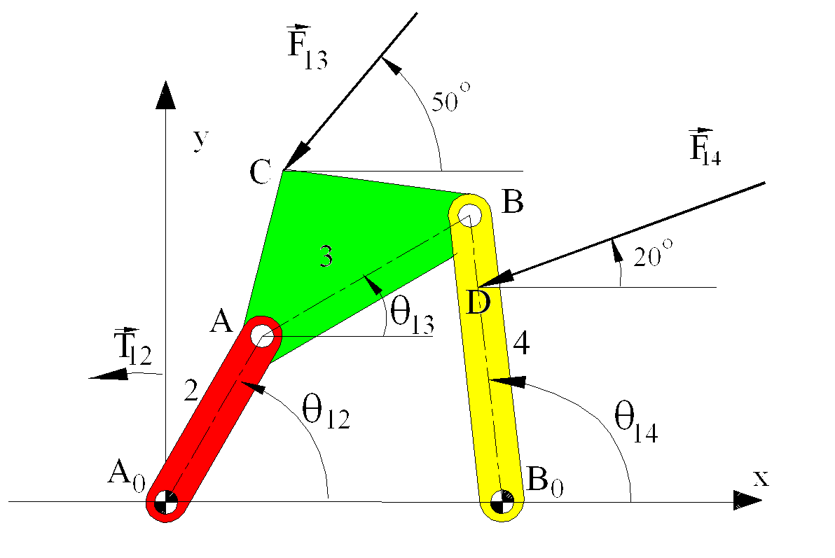
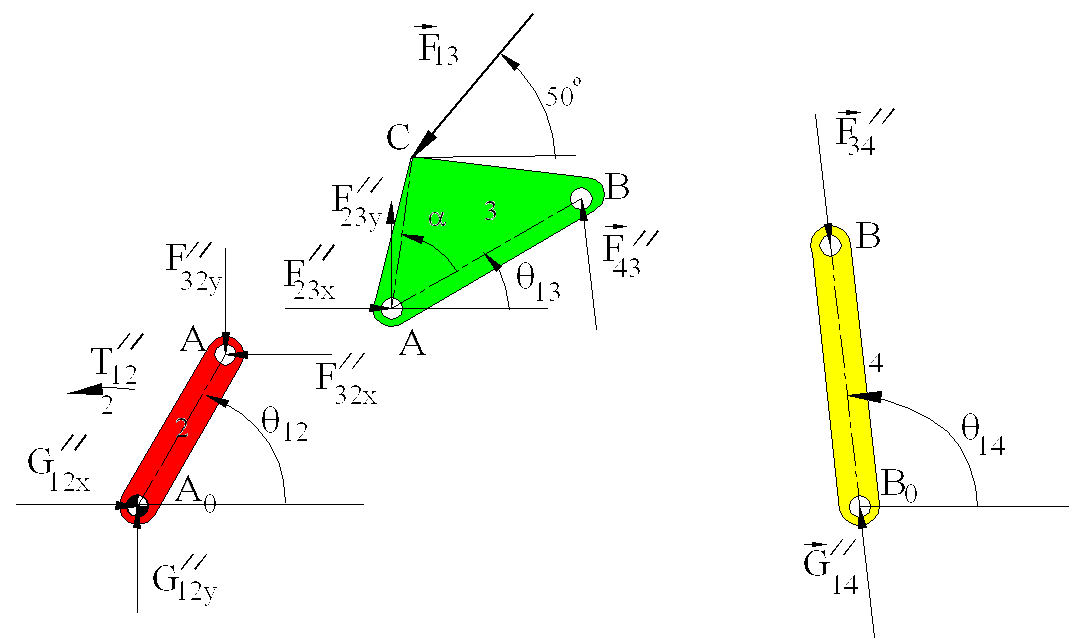
For the mechanism shown |A0A| = a2 = 80, |AB| = a3 = 100, |B0B| = a4 = 120, |A0B0| = a1 = 140, |AC| = b3 = 70, |BC| = 80 and |B0D| = b4 = 90 mm. When θ12 = 60°, from kinematic analysis θ13 = 29,98°, θ14 = 96.40°. Two forces F13 = 50 N ∠230° and F14 = 100 N ∠200° are acting on links 3 and 4 respectively.
Solution without the principal of superposition
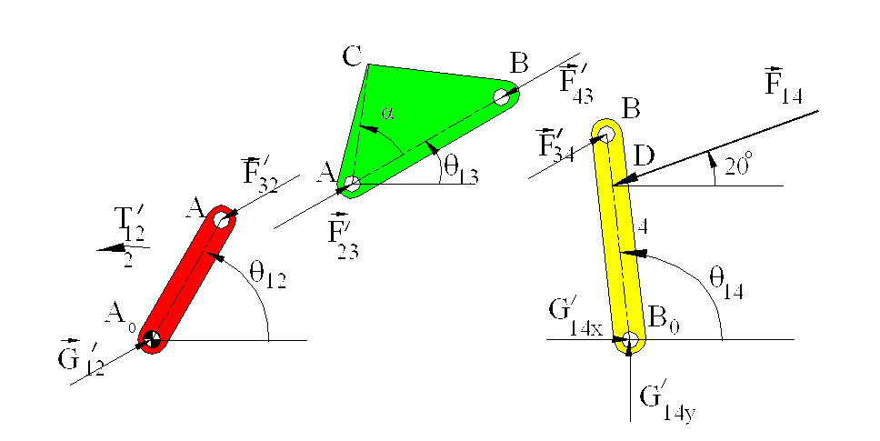
The free-body diagrams of the moving links are shown. The three equilibrium equations for link 4 are:
| SFx = F34x + G14x − F14 cos20° = 0 | (1) |
| SFy = F34y + G14y − F14 sin20° = 0 | (2) |
| SMB0 = −a4 F34x sinθ14 + a4 F34y cosθ14 − b4 F14 sin(20° − θ14) = 0 | (3) |
There are four unknowns in three equations, therefore the equations obtained from one free-body diagram is not enough to solve for the unknowns. Equations 1 and 2 can be used to solve for G14x and G14y, only when F34xy and F34y are determined. The three equilibrium equations for link 3 must also be written (note that F34 and F43 have equal magnitude).
| SFx = F23x − F34x − F13cos50° = 0 | (4) |
| SFy = F23y − F34y − F13sin50° = 0 | (5) |
| SMA = a3 F34x sinθ13 − a3 F34y cosθ13 − b3 F13 sin(50° − θ13 − α) = 0 | (6) |
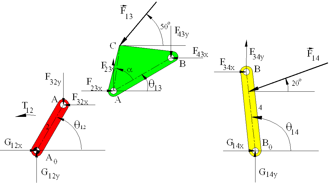
where α = 52.62° (using the cosine theorem for triangle ABC). Equations 4 and 5 can be used to determine F23x and F237x. Equations 3 and 6 must be used simultaneously to solve for F34x and F34y. Substituting the known values into equations 3 and 6 results:
| −119.25 F34x− 13.38 F34y + 8748 = 0 | (3) |
| 49.97 F34x – 86.62 F34y + 1886 = 0 | (6) |
Simultaneous solution of the two equations yield:
F34x = 66.60 N F34y = 60.20 N F34 = 89.78 N ∠42.11°
From equations 1 and 2:
G14x = 27.37 N G14y = 26.00 N G14 = 37.75 N ∠−43.53°
From Equations (4) and (5):
F23x = 98.74 N F23y = 98.50 N F23 = 139.46 N ∠44.93°
Now, link 2 can be treated as a two force and a moment member (G12 = −F32 = F23). The moment equilibrium (about A0):
T12 − a2 F23 sin(47.34° − 60°) = 0 or T12 = −2908 N·mm = 2.9 N·m (CW)
Solution using the principal of superposition
The same problem will be solved usiing the principle of superposition. Let us consider two problems:
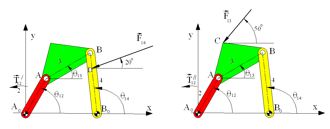
In problem (a) the mechanism is under the action of F14 and in (b) F13 only. If we denote the joint forces due to F14 by a single prime and the forces due to F13 by double prime, we have the free-body diagrams due to F14 as shown:
Due to F14, the moment equilibrium for link 4 yields:
a4 F′34 sin(θ13 − θ14) − b4 F14 sin(20° − θ14) = 0
from which F′34 = 79.54 N ∠29.98° (= θ13).
Since F′34 = −F′43 = F′23 = −F′32 = G′12 (links 3 and 2 are two-force and two force and a moment members respectively ; also action-reaction between bodies 2, 3, 4), we have to write the moment equilibrium for link 2 only:
T′12 − a2 F′32 sin(θ13 − θ12) = 0
from which T′12 = −3184 N·mm = 3.18 N·m (CW)
Due to F13 only:
Link 4 is a two-force member, link 3 is a three force member while link 2 is a two-force and a moment member as before. The moment equilibrium equation for link 3 yields:
a3 F″43 sin(θ4 − θ13) − b3 F13 sin(50° − θ13) = 0
from which F″43 = −20.57 N ∠96.40° (= θ14) or F″34 = −F″43 = 20.57 N ∠96.40°
F″23x and F″23y can be determined using the force equilibrium equations for link 3:
F″23x = F13 cos50° + F″43 cos(θ14) = 29.85 N
F″23y = F13 sin50° + F″43 sin(θ14) = 58.74 N
F″23 = 65.89 N ∠63.06°
Now, the moment equilibrium for link 2 yields:
T″12 − a2 F″32 sin(63.06° − θ12) = 0
from which: T″12 = 282 N·mm = 0.28 N·m (CCW)
One can now superimpose the two solutions. For example, the torque T12 required for the original system will be:
T12 = T′12 + T″12 = −3184 + 282 = −2902 N·mm = 2.9 N·m (CW)
Similarly:
F34x = F′34x + F″34x = 79.54 cos(29.98°)+ 20.57 cos(96.40°) = 66.60 N
F34y = F′34y + F″34y = 79.54 sin(29.98°)+ 20.57 sin(96.40°) = 60.19 N
F23x = F′23x + F″23x = 79.54 cos(29.98°) + 29.85 = 98.75 N
F23y = F′23y + F″23y = 79.54 sin(29.98°) + 58.74 = 98.49 N
F23 = G12 = 139.5 N ∠44.92°
F34 = 89.77 N ∠42.11°
The results are in good agreement with the results obtained previously (small differences are due to the round-off errors).
Different formulations can be used depending on the type of the problem to be analysed, on the accuracy required, time to be spend and the available numerical computation facilities. For example, if a rough estimate is to be made for one particular position, a graphical computation may be the simplest (whether done by drafting instruments or by a drawing program). If the problem is to be repeated over and over for different positions and for different external load conditions (and maybe with different link lengths) a general formulation and writing a general computer program for the machine will be more feasible. If different types of structures are to be investigated in a development stage, use of a package program such as Working Model® or ADAMS® may be useful. Usually an engineer must check his results by performing the same computation in two or more different ways.
![]()
![]()
![]()
![]()
![]()