3.4 Vector Loops of a Mechanism

The main difference between freely moving bodies and the moving links in a mechanism is that they have a constrained motion due to the joints in between the links. The links connected by joints form closed polygons that we shall call a loop. The motion analysis of mechanisms is based on expressing these loops mathematically.

In kinematic analysis we shall assume that all the necessary dimensions of each link is given and link length dimensions (i.e. the distance between the joints or the angles) can be determined from the given dimensions using the geometry of the link.

In Section 2.1.2, we have seen that it is sufficient to represent the position of each link (rigid body) by describing the position of any two points on that link. One way of selecting these two points on a link is to use the permanently coincident points. It is obvious that in such a procedure, the origin of a vector will be defined by the previous vector and thus the number of parameters to define the link positions will be decreased.

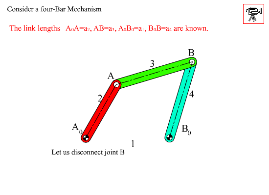
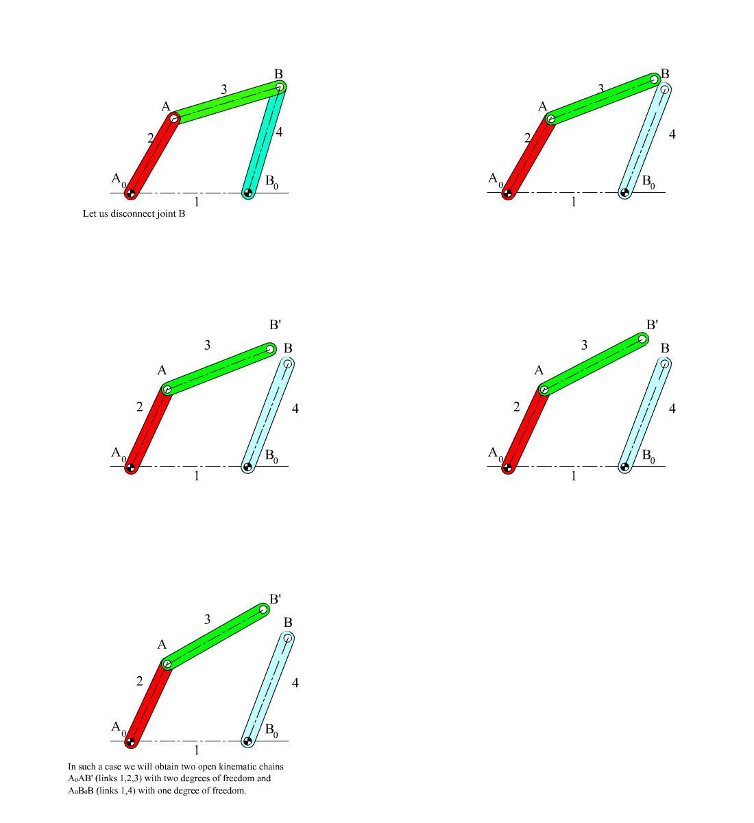
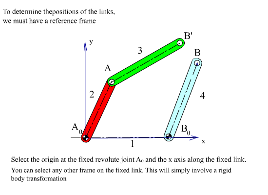
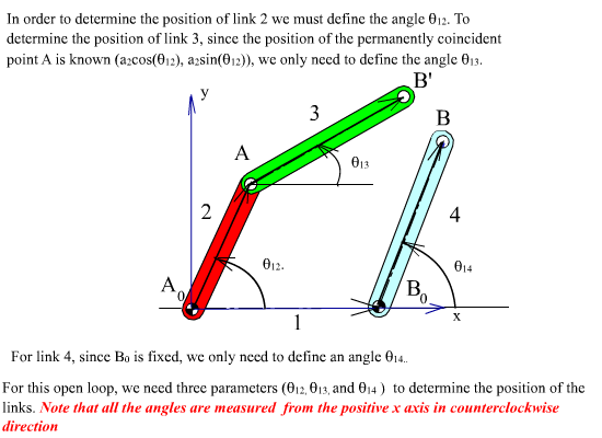
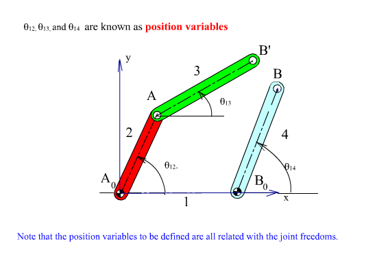
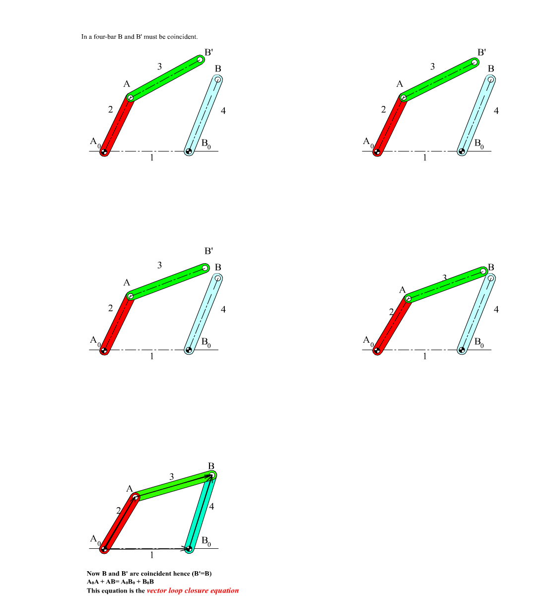
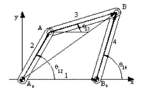
Let us consider a four-bar mechanism as shown above as a simple example. In this mechanism A₀ ,is a permanently coincident point between links 1 and 2, A is peranently coincident point between links 2 and 3, B between 3 and 4 and B₀ between 1 and 4. Let us disconnect joint B. In such a case we will obtain two open kinematic chains A₀AB (links 2, 3) with two degrees of freedom and A₀B₀B (links 1, 4) with one degree of freedom (see figure). To determine the positions of the links we must have a reference frame. One obvious choice is to select the fixed pivots A₀, B₀ as one of the co-ordinate axes and select A₀ or B₀ as the origin. Next,in order to define the position of link 2, we must define angle θ₁₂, which is related with the degree of freedom of the joint between links 1 and 2. To determine the position of link 3, since the location of the permanently coincident point A between 2 and 3 can be determined when θ₁₂ defined, we must now define θ₁₃ , which is related to the freedom of the joint between links 2 and 3. Similarly θ₁₄ must be defined to determine the position of link 4. Hence we need 3 parameters (θ₁₂, θ₁₃ and θ₁₄ ) which are all related to the joint freedoms for the open kinematic chains obtained when we disconnect a joint to eliminate a loop.

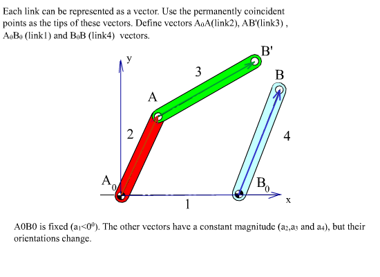
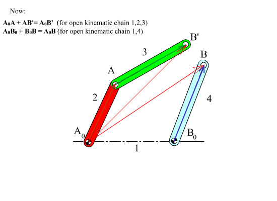
Each link can be defined by a vector fixed on that link, let us select the permanently coincident points between the links as the tips of these vectors and define vector A₀A (for link 2), AB (for link 3), B₀B (for link 4) and A₀B₀ (for link 1). Except A₀B₀ , the other three vectors will be a function of time (since the distances between the two points on the same link are fixed, the magnitudes will remain constant but the directions of these vectors will change in time). Since the mechanism contains revolute joints only, The magnitude of the vectors are constant link lengths (a₂ = |A₀A|, a₃ = |AB|, a₁ = |A₀B₀| and a₄ = |B₀B|). The angular orientation of these vectors will be rotation variables (θ₁₂, θ₁₃ and θ₁₄ ). When the joint at B is disconnected, B₃ and B₄ may not be coincident. For the open kinematic chain, the position of point B may be defined in two different forms as:

A₀A + AB = A₀B₃ (1, 2, 3 open loop)

A₀B₀ + B₀B = A₀B₄ (1, 4 open loop)

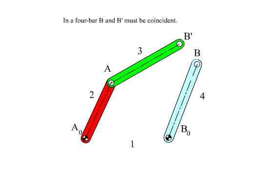
However, at every instant the revolute joint between links 3 and 4 must exist and point B must remain a permanently coincident point for different values of the position variables if the system we are considering is a mechanism. Therefore the vector A₀B₃ and A₀B₄ obtained from the two equations using the two open kinematic chains must be equal and this results with the vector equation:

A₀A + AB = A₀B₀ + B₀B

This vector equation must be valid for all positions due to the permanetly coincident points. If this vector equation can nott be satisfied for a given input angle, then that position cannot exist (mechanism cannot be assembled at that position).

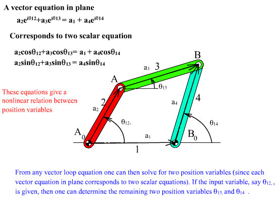
In a four-bar mechanism there is a single loop formed and the vector equation describes the closure of this loop mathematically.The equation(s) that describes the closure of the loop(s) formed in the mechanism are known as loop closure equation(s). The variables in the loop closure equations are always related by the joint freedoms and we can solve for two position variables from any loop equation. In plane the vector equation will correspond to two scalar equations. In the four-bar example there are three variables (θ₁₂, θ₁₃ and θ₁₄) which we shall call “position variables“. If one of the position variable (say θ₁₂), the other position variables (θ₁₃ and θ₁₄) can be solved from this vector loop equation. The number of independent parameters that are required will always be equal to the degree-of-freedom of the mechanism. The relation between the position variables is a nonlinear, trigonometric relation.

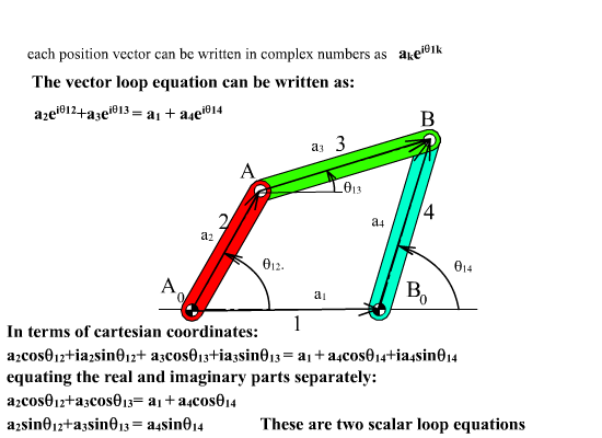
One simple and concise form of writing the vector loop equations is to use complex numbers. for example, If the length of the vector A₀A is a₂ and if the vector makes an angle θ₁₂:

A₀A = a₂cosθ₁₂ + ia₂sinθ₁₂

or, using Euler’s equation:

A₀A = a₂e^iθ₁₂

In a similar fashion if the link lengths are denoted as a_i olarak (a₁= |A₀B₀|, a₂=|A₀A|, etc.) the vector loop equation in complex numbers can be written as:

a₂e^iθ₁₂ + a₃e^iθ₁₃ = a₁ + a₄e^iθ₁₄

If required, the equation can be written in cartesian coordinates as:

a₂cosθ₁₂i + a₂sinθ₁₂j + a₃cosθ₁₃i + a₃sinθ₁₃j = a₁i + a₄cosθ₁₄i + a₄sinθ₁₄j

x and y components can be equated separetely two yield two scalar equations in the form:

a₂cosθ₁₂ + a₃cosθ₁₃ = a₁ + a₄cosθ₁₄
a₂sinθ₁₂ + a₃sinθ₁₃ = a₄sinθ₁₄

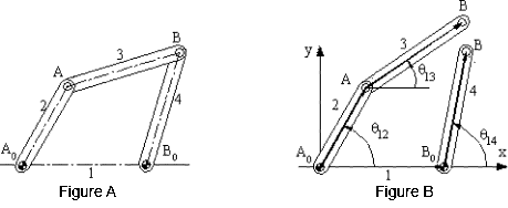
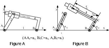
In case of a four-bar, the vectors in the loop closure equation have fixed magnitudes. However, the angular inclinations of the three vectors representing the moving links will change. Hence, there are three position variables (θ₁₂, θ₁₃ and θ₁₄). If one of these variables is defined, the remaining two variables can be solved from the vector equation. If we refer to the definition of the degree-of-freedom of a mechanism, the variable that must be defined is the input variable and for a constrained motion the number of input variables must be equal to the degree-of-freedom of the joints involved. In case of a four-bar, since all the connections are revolute joints, the variables are all rotation variables. In case of a prismatic joint, the variable will be the magnitude of a vector or a vector component. Consider a slider-crank mechanism as shown in Fig. A. Let us disconnect the revolute joint at B (Fig. B). In order to determine the positions of links 2 and 3 we must define θ₁₂ and θ₁₃. To locate the position of link 4 its displacement along the slider axis must be known and the position variable s₁₄ must be defined. The resulting loop closure equation is:

A_oA + AB = A_oB

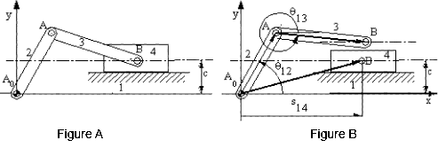
Again there are 3 variables (θ₁₂, θ₁₃ and θ₁₄) one of which must be specified as the input. In this case the vectors A_oA and AB have fixed magnitudes and varying directions. The vector A_oB has a fixed y component (length c) and a changing x component (s₁₄). Depending on the applications either θ₁₂ (i.e. in pumps) or s₁₄ (i.e. internal combustion engines) is the input. In complex numbers the vector loop equation will be:

a₂e^iθ₁₂ + a₃e^iθ₁₃ = s₁₄ + ic

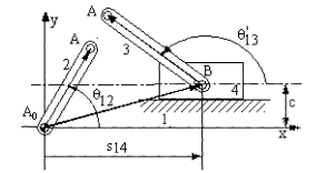
The vectors defined and the variables used in the loop closure equations are not unique. For example, for the slider crank mechanism, rather than disconnecting the revolute joint at B, one can as well disconnect the revolute joint at A between links 2 and 3 (Fig C). We must now define the angle θ₁₃′ = ∠xBA instead of the angle θ₁₃ o determine the position of link 3. Note that the angles. θ₁₃ and θ₁₃′ differ by a constant angle (In this case by 180^o). The resulting loop equation is:

A_oA = A_oB + BA

or in complex numbers:

a₂e^iθ₁₂ = s₁₄ + ic + a₃e^iθ₁₃′

Example: The loop closure equations of a six link mechanism

Referring to the four-bar mechanism above, one can write a vector equation in the form:

A_oA + AB = A_oB

Considering the vector A_oB the magnitude and direction of this vector are variables (or its x and y components) and these variables are not related with the joint freedoms.we can solve for the vector A_oB provided that the magnitudes and the directions of the other two vectors are known. Such an equation will not help us for the solution of position variables. Although it is a valid vector equation, it is not a loop closure equation. One can identify such loops by noting the variables involved are not related with the joint freedoms and these equations are not obtained by disconnecting the joints.

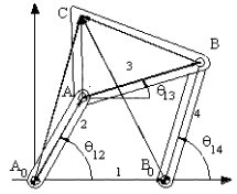
A similar argument can also be made for the vector equations:

A_oA + AC = A_oC         (i)

AB + BC = AC         (ii)

In the later case, all three vectors are on the same link and they have a fixed orientation with respect to each other. If the origin and the angular orientation of one of the vectors is known, due to rigidity the orientation of the other vectors will be known.

In certain other cases we may have to use instantaneously coincident points or other points on the links as the tips of the vectors, as shown in the figure. The variable involved in such a case is the relative displacement of one link with respect to another link. The vector B_oA can be separated into two components: B_oC and CA so that one component is of constant magnitude and the magnitude of the other vector is related to the displacement of the prismatic joint between links 3 and 4. The loop closure equation can than be written in the form:

A_oA = A_oB_o + B_oC + CA

or in complex numbers:

a₂e^iθ₁₂ = a₁ + a₄e^iθ₁₄ + s₄₃e^{i(θ₁₄ + α₄)}

Points A₂ ve A₃ are permanently coincident points. Point A₄ is instantaneously coincident with point A₃ when the mechanism is moved from this position the two points will be displaced by a distance Δs along the slider axis relative to each other. Points A₂ and A₃ will be two other different points that will be coincident with (A′) (Fig. C).

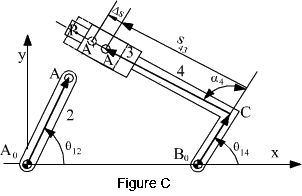
The vector CA changes both its magnitude and direction. However its orientation with respect to the vector B₀C will be fixed, and no new variable is needed. If the orientation of the vector B₀C is whown by the variable θ₁₄ measured from the positive x-axis of our reference, the orientation of the vector CA with respect to positive x axis is θ₁₄ + α₄ and angle α₄ is a constant angle measured on link 4 between two lines B_oC and CP (point P is any point on the slider axis on link 4). The position variables in the loop equation will be θ₁₂, θ₁₄ and s₄₃.

Note that the same vector loop equation can be derived for the swinging block mechanism shown above. Therefore, the inverted slider crank mechanism is the same as the swinging block mechanism although their construction is different. Although it is a different construction, if the link dimensions (a₂, a₄, α₄) are the same, the motion of the two mechanisms will be the same.

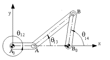
When writing the vector loop equations one must be sure that the equations are valid for every position of the mechanism. The mechanism may be at a special position such that one or more of the links are collinear as shown above (Although links 2 and 1 are collinear, they will have different orientations at some other instant). In such a case you may redraw the mechanism slightly offset from the critical position or show the variable angle θ₁₂, as shown. In some cases if the constant link angles between two vectors are of a certain simple value (such as 90°), then it is advisable to simplifiy the equations accordingly. For example if the angle α₄ of the inverted slider crank mechanism is a right angle, The loop closure equation must be written as:

a₂e^iθ₁₂ = a₁ + a₄e^iθ₁₄ + is₄₃e^iθ₁₄

The solution to the loop equations may not exist for every value of the independent parameter. This will mean that for that particular link lengths the mechanism cannot be assembled at the requested position.

How will you determine the number of independent loops from the number of joints and links?

In planar mechanisms we can write vector loop equations for each loop of the mechanism. This corresponds to L (L= number of independent loops) vector equations or 2L scalar equations, if we equate the x and y components of vectors. The number of parameters involved in these equations will be 2L+ F, where F is the degree of freedom of the mechanism. If we now define F number of variables (independent variables or input parameters (variables)), then theoretically, we must be able to solve for the other variables (dependent position parameteres). We can change the input variable within a given range in certain increments and obtain the values for the dependent variables. For example if the input variable corresponds to the angle that defines the angular position of an input crank, we change this angle from 0 to 360^o. If the input is the movement of a piston inside a cylinder, then we change this length of the piston starting from the closed position to the most extended position (the difference is the stroke of the piston).

When we determine the values of all the position variables corresponding to a certain input variable, then we can determine the position of any point on any link of the mechanism.

One need not draw the mechanism with dismantled joints to write the loop equations. After some practice one can conceptually disconect the joints, identify the loops and the write the necessary loop equations. Initially of course, as a visual aid, we have shown the joints are shown disconnected.

In the following examples the necessary loop equations for some mechanisms are written. The loop equations and the variables defined are not unique. You are to determine the joint that is disconnected when writing the given loop equation.

In recent years different package programs are available for the analysis of mechanisms. When using these programs, you must input these loops by telling the program which link is connected to which link by what kind of a joint (i.e. what kind of freedom is permitted by that joint). If you are using mathematical packages such as matlab or mathcad, you must type these equations in one form or another. A slight mistake in the loop equations results with erroneous results. Please keep in mind that these equations define the mathematical model of an existing mechanism. This mathematical model can be solved in different ways as we shall see in the coming sections.

Example I:

(a₂ = |A₀A|, a₃ = |AB|, a₄ = |BC|)

A₀A + AB + BC = A₀C  ⇒  a₂e^iθ₁₂ + a₃e^{i(θ₁₃ − α₃)} + a₄e^iθ₁₄ = s₁₅ + ia₁

A₀A + AD = A₀D₀ + D₀D ⇒  a₂e^iθ₁₂ + s₃₆e^iθ₁₃ = c₁ + ib₁ − ia₆e^iθ₁₃

Example II:

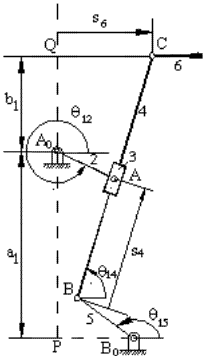
(c₁ = |PB₀|, a₂ = |A₀A|, a₄ = |BC|, a₅ = |B₀B|)

A₀A = A₀B₀ +B₀B + BA  ⇒  a₂e^iθ₁₂ = c₁ − ia₁ + a₅e^iθ₁₅ + s₄₃e^iθ₁₄

A₀C = A₀B₀ + B₀B + BC  ⇒  s₁₆ + ib₁ = c₁ − ia₁ + a₅e^iθ₁₅ + a₄e^iθ₁₄

Example III:

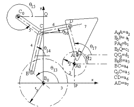
B₀B + BC + CD = B₀A₀ + A₀A + AD  ⇒  a₃e^iθ₁₃ + a₄e^iθ₁₄ + a₆e^iθ₁₆ = a₁ + ib₁ + a₂e^iθ₁₂ + a₇e^iθ₁₇

B₀B + BC = B₀C₀ + C₀C  ⇒  a₃e^iθ₁₃ + a₄e^iθ₁₄ = −d₁ + ic₁ + a₅e^iθ₁₅

Due to the gear pair : r₃θ₁₃ = −r₂(θ₁₂ − α₂) (θ₁₂ = α₂ when θ₁₃ = 0)