4.2 VELOCITY AND ACCELERATION ANALYSIS OF MECHANISMS-5

Example:

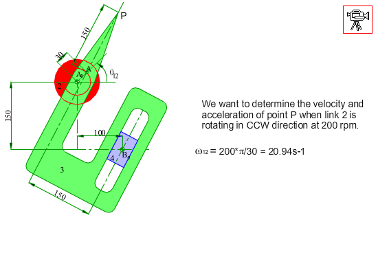
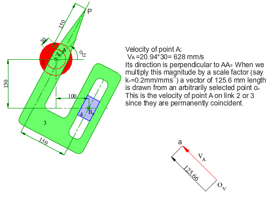
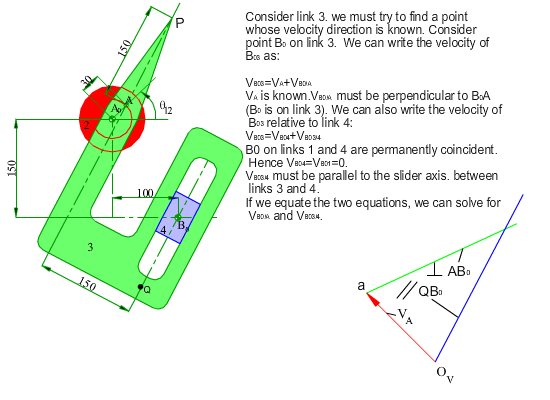
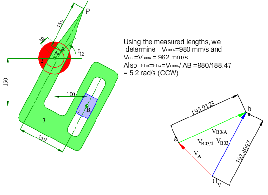
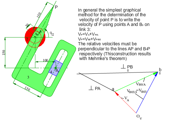
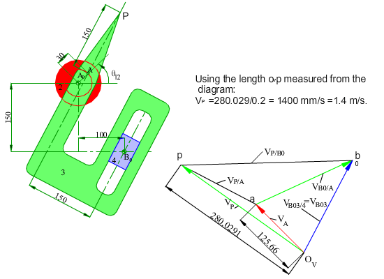
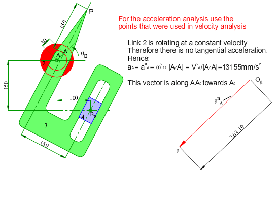
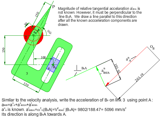
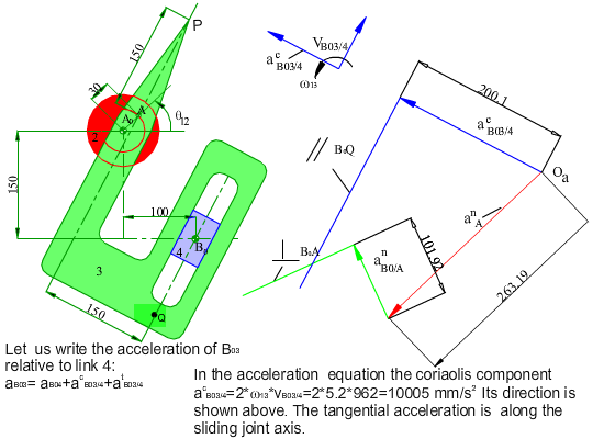
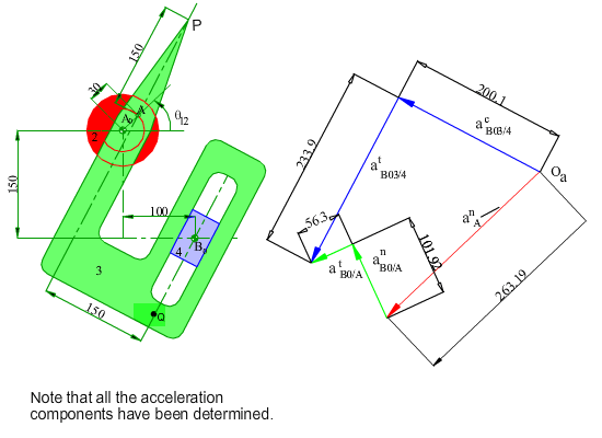
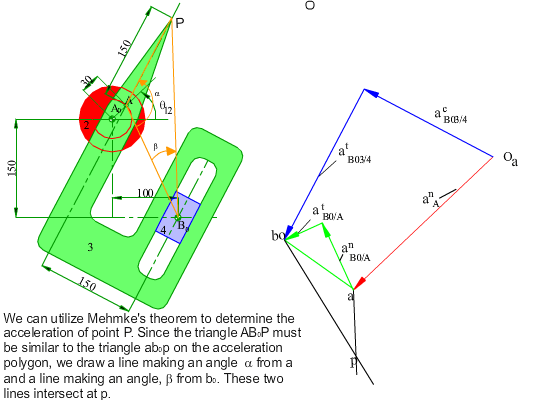
In the figure shown, the crank (link 2) of the mechanism rotates at a constant speed of 200 rpm counter clockwise. Determine the velocity and the acceleration of point P for any input crank angle θ₁₂. First a graphical solution for a particular position will be shown. Next an analytical solution for every crank angle will be discussed.

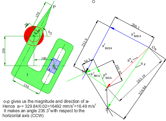
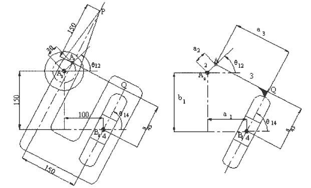
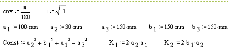
In case of the analytical solution, the main problem is the identification of the loop and the position variables.  If we redraw the mechanism as in figure (b) below, the identification of the position variables may be more obvious. The most important rule is that one must disregard the shape of the links and concentrate on the joints involved. In such a case we can write the loop equation in complex numbers as:

a₂e^iθ₁₂ = a₁ − ib₁ + s₄₃e^iθ₁₄ + ia₃e^iθ₁₄

Using the method shown in the previous sections, the loop equation can ve solved for the unknown position variables (θ₁₄ and s₃₄), and the loop equation can be differentiated to obtain the velocity and acceleration loop equations which can be solved for the unknown velocity and acceleration variables.

a) Orijinal Shape                                                b)  Equivalent Schematic drawing

The Mathcad solution for this problem is as follows. Define the constants:

Change the input crank angle for every degree:

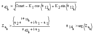
Determine the position variables s₃₄ and θ₁₄:

Determine the position of point P and plot it:

Velocity Analysis

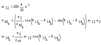
For the acceleration analysis the above equations are differentiated with respect to time directly (note that you cannot correlate the acceleration components with the terms in these equations).

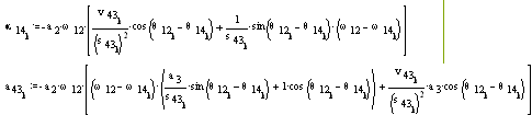
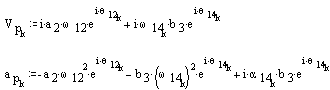
Now, the velocity and acceleration of point P can be determined.

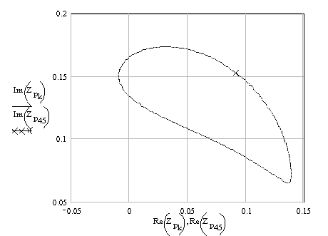
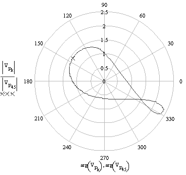
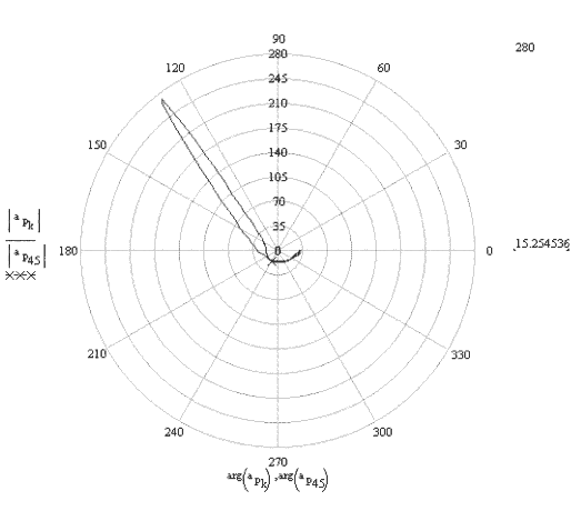
The polar plot of the velocity and acceleration of point P for one cycle are shown below.