CENG 587 HW1: Recovering Camera Response Curves with Debevec & Malik

Yiğit Alp Dalyan, 12/11/2026

Contents

1. Introduction
2. The Algorithm
3. Implementation
4. Difficulties and Solutions
5. Validation on the Virtual Camera
6. Effect of Lambda
7. My Phone’s Camera Response Function
8. Running Times
9. Conclusion
10. References

1.Introduction

Most cameras in use can only capture a limited dynamic range when capturing images. This limited dynamic range is generally only a fraction of the actual dynamic range present in many physical scenes, or what we can actually see with our eyes. Vast majority of published methods to capture the full dynamic range of the scene using regular low-dynamic-range cameras relies on shooting multiple frames at different exposures to capture a different section of the scenes dynamic range, and then blend these frames to generate the full range of the scene.

However, some blending methods require the actual exposure that is captured at each pixel. This poses a problem as the final output of many digital cameras (and film processing-scanning of film cameras) introduce strong non-linearities to the mapping between actual sensor pixel exposures and digital image pixel values.

The actual function between the sensor exposure value and the image pixel value is called the Camera Response Function (CRF). The CRF is required by many HDRI papers that require the actual exposures that generate the pixel values in digital images.

For HW1 I implemented to calculate the CRF of my phone is the one proposed by Debevec and Malik (1997). I also ran the supplied virtual camera brackets through my implementation and compared the resulting CRF with the simulated CRF of the virtual camera. Finally I ran the implementation with different lambda smoothing constant values to see its impact on the generated CRF.

2. The Algorithm

The algorithm relies on the regular exposure relation:

where g is the log-inverse CRF, E_i is the desired irradiance at the sensor pixel, and delta t_j is the exposure time used for the image capture.

Debevec and Malik proposed that, as g is a function mapping discrete values of Z [0-255] to exposure values, and there are a finite amount of pixels with unknown irradiance values, the exposure relation can be seen as a system with (Z_max – Z_min) + N unknowns, with N x P equations, where N is the number of sampled pixels, and P is the number of images in a bracket. This system can be solved by writing out an objective function, and minimizing it.

g”(z) is the second difference function that adds a smoothing factor that minimizes the second derivative of the generated inverse-CRF.

And omega is the hat weighting function that gives more weights to pixels with values closer to 128 when generating g, and blending for the final irradiance-map.

The generated CRF is ambiguous to the additive constant, as a constant value added to both g(Z) and log-E will cancel each other in the objective function. Therefore the g(128) is fixed to 0.

As there are (Z_max – Z_min) + N unknowns, and N x P equations, and N x P must be greater then (Z_max – Z_min) + N for this system of equations to be solvable, the following sampling condition applies for the Debevec and Maliks method. This means at least 43 samples are required for my common phone bracket case of 7 exposures and 256 Z range.

3. Implementation

The implementation was done as a single python script, each step implemented as a function, and the pipeline was implemented by chaining the functions together. Numpy and OpenCV were used for image processing, Pillow with the pillow-heif module were used for image import. Matplotlib was used for graphing.

The implementation pipeline is as follows:

1. The brackets were loaded one-by-one using pillow+pillow-heif. EXIF information was used for the exposure times in the algorithm. The brackets were then checked for single-ISO and common size, and sorted by the exposure times.
2. The brackets were then downscaled by 0.1x using the OpenCV resize method with INTER_AREA method for the phone brackets, resulting in brackets with 403×302 resolutions. The virtual camera brackets resized to 500px wide images.
3. The median image in the bracket was selected as the reference image, converted to grayscale, OpenCV Sobel method was used to generate the gradient of it, and the below median gradient points were masked as possible candidates. The brightness range was separated to 16 bins, and the 200 points were distributed to each bin uniformly. Then the points in the low-gradient mask with the wanted brightness were selected randomly for each bin. Due to an implementation quirk (200 integer division to 16 equals 12, 12×16=192). 192 samples were actually selected, but 192 samples proved enough for the chosen brackets.
4. Z matrix was built per channel, and the numpy lstsq least squares solver was used to solve the system. A matrix size was (NxP + 255) x (256 + N). with 7 image brackets and 192 sample the A matrix size is 1599×448.
5. The bracket was merged to a radiance map using Debevec and Maliks method with the hat weighting function, and saved as a .hdr file. The radiance map was also tone mapped with Reinhard using OpenCV’s createTonemapReinhard method.

The sampling method tries to minimize the overrepresentation of common brightness regions in the image, however if the other bins are empty the total sample count may be less then 192. Phone bracket 121644 gave 144, virtual camera srgb image gave 146, and linear image gave 107 samples. However all of these were above the methods condition of 43 minimum samples.

4. Difficulties and Solutions

• Some exposure-brackets I captured with constant ISO settings ended up with mixed ISO speeds as the darker exposures hit the 1/40000 limit of my phone sensor, so I had to exclude them.
• I had to cast pixel values to int64 when generating the Z matrix for the least squares solver to avoid a uint8 overflow.
• When comparing virtual camera curves with the ground truth I had to align the curves by calculating an offset using the means of the curves weighted by the hat function.
• Default settings of the Reinhard tone mapper in OpenCV resulted in tone-mapped images that were too bright and washed-out for the brackets of my scenes. I had to use light_adapt=0 to turn off local pixel adaptation, and add a negative intensity bias of -1.

5. Validation on Virtual Camera

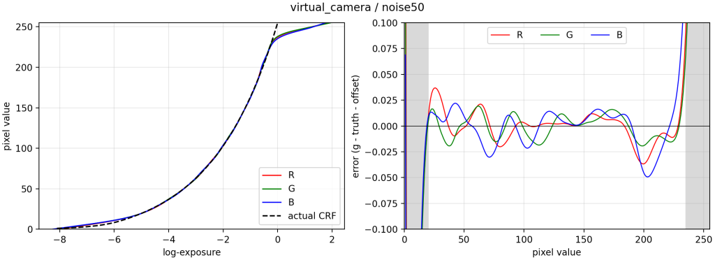
Virtual camera brackets are renders in HW1 handout from the Greg Ward’s Radiance ray-tracer, captured with linear and sRGB response functions, and added noise. The brackets are captured with 1-stop exposure separations.

The ground truth log-exposure values captured by the virtual camera is then the log of the inverse sRGB function. The offset between the means of the log-exposures of the inverted pixel values and ground truth is removed to eliminate the constant offset of the method. The error statistics were then calculated using the region 20-235 to prevent the impact of clipping noise.

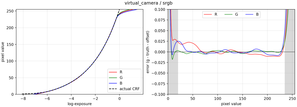
Channel	RMS (log)	Max (log)
R	0.0103	0.029
G	0.0035	0.026
B	0.0083	0.052

6. Effect of Lambda

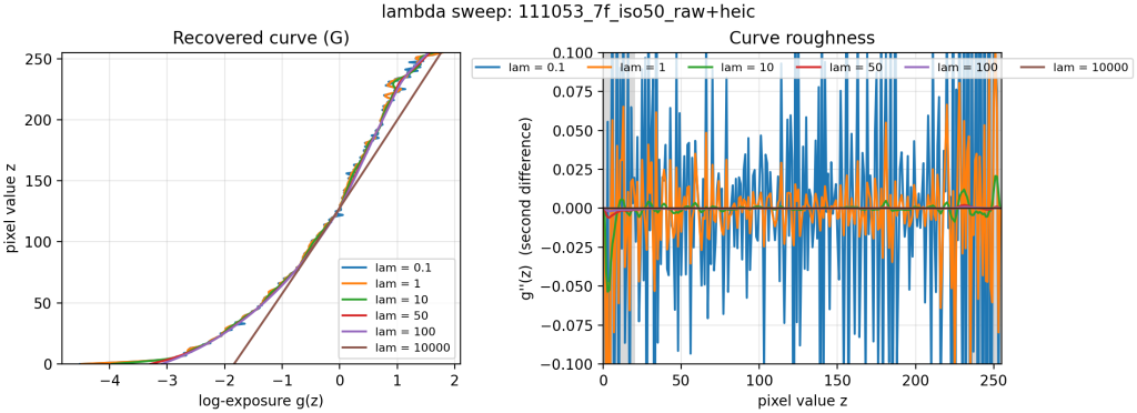
Small lambda values cause spikes in the second derivative of the generated G curve, especially to the edges of the curve as the relevant sample count drops, pixels saturate at the bright end, and noise dominates at the dark end.

High lambda values like 10000 cause the curve to over smooth, and results in a curve that is a linear line in log-exposure.

Lamda value was chosen as 50 as it was the first lambda value that resulted in nearly zero g” spikes while still correctly fitting the camera CDF.

7. My Phone’s Camera Response Function

Capture

• All the exposure-brackets were shot using the main camera of my iPhone 17’s main camera, 5.96mm f/1.6
• I used the ProCamera app to capture brackets. The constant ISO setting was used to generate exposures with only exposure time varying between them, as assumed by the algorithm.
• The brackets were shot at Soğuksu National Park in an Overcast day.
• Each bracket consists of 7 exposures, with varying exposure ratios.

Data Cleaning

I captured 20 brackets, but I could only use 12 of them to test my implementation as 8 of the brackets had its lower exposures hit the 1/40000 exposure time limit of my phone and used lower ISO speeds to achieve lower exposures. This broke the algorithm’s constant-ISO assumption.

Recovered Curves

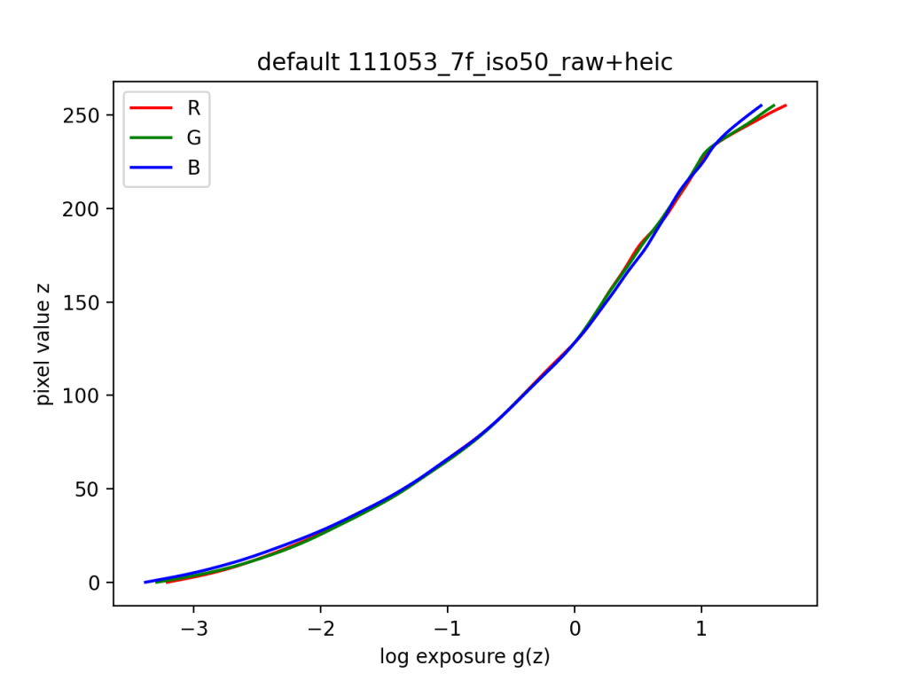
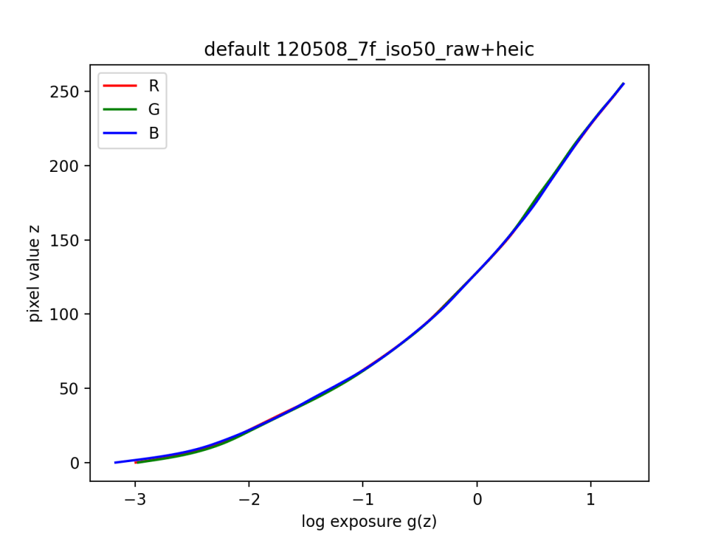
The curve rises slowly for the shadows (z < 50). For the midtones the CRF curves follow a linear line in log-exposure, indicating that they are following a logarithmic mapping from the pixel exposures, equal exposure-stop increases map to equal increases in pixel value. For the highlights, the curve bend and flattens. This is more noticeable on the curve extracted from the bracket 111053 as it has more highlight information in the brackets than 120508. Each channels CRF is nearly identical.

The curves also show that the CRF is indeed non-linear as a linear mapping would look like an exponential curve with the log-exposure axis.

HDR Result

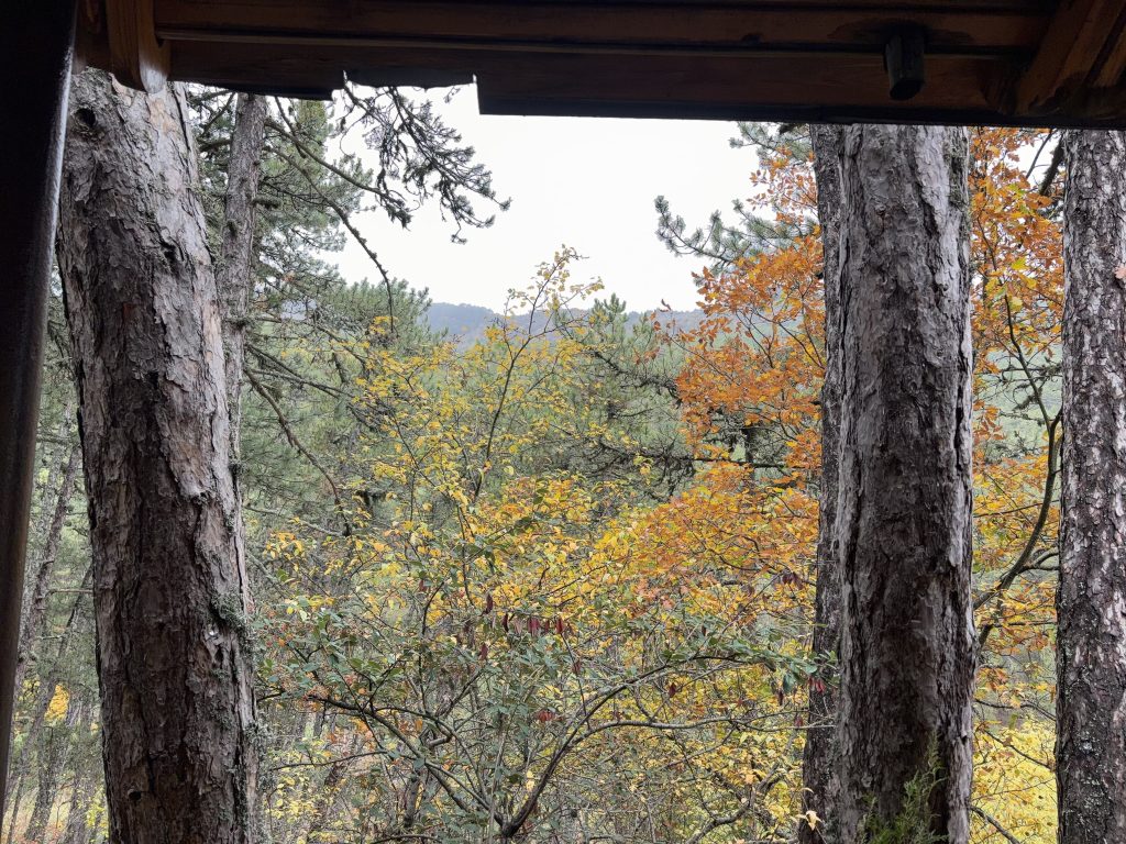
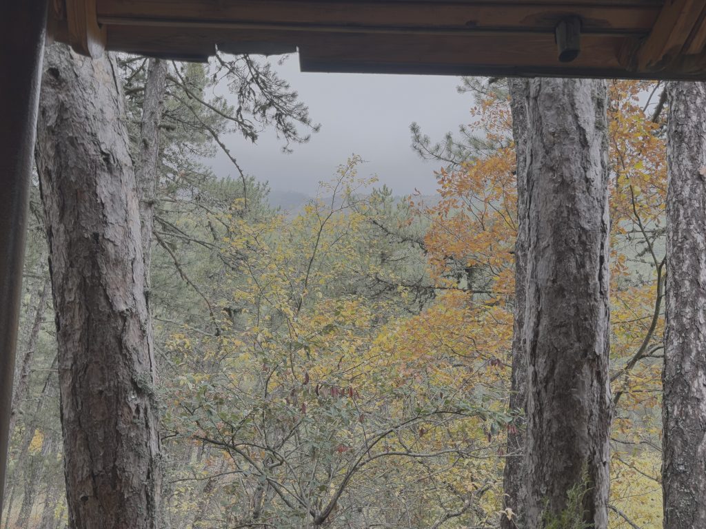
The HDR result captures the sky features and the wood grain details in the scene. Due to the nature of a overcast scene acting like bright but uniform illumination there isn’t much high-dynamic-range features in the ground, however the overall dynamic range of the scene was still around 6.5 stops.

8. Running Times

Timings were measured on a MacBook Air (Apple M5, 16 GB RAM), macOS 26.5.2, Python 3.9.6, NumPy 2.0.2, OpenCV 5.0.

Dataset	N	P	Size	Sampling (ms)	Solve R (ms)	Solve G (ms)	Solve B (ms)
105052_7f_iso100_heic	192	7	403×302	28.8	19.6	19.2	18.2
105340_7f_iso64_heic	192	7	302×403	7.1	19.4	19.2	19.5
105945_7f_iso80_heic	192	7	302×403	6.5	20.3	19.0	18.4
110622_7f_iso160_heic	168	7	403×302	7.1	15.0	14.5	14.7
110655_7f_iso50_heic	192	7	403×302	6.6	19.2	19.2	19.4
111053_7f_iso50_raw+heic	192	7	403×302	6.3	19.0	19.3	19.3
111120_7f_iso80_raw+heic	192	7	302×403	7.1	19.6	19.4	19.4
111219_7f_iso40_raw+heic	163	7	302×403	6.5	14.6	14.1	13.8
120508_7f_iso50_raw+heic	192	7	302×403	5.8	19.5	19.1	19.2
121644_7f_iso64_raw+heic	144	7	403×302	6.4	13.7	13.8	13.7
122523_7f_iso50_raw+heic	192	7	403×302	6.6	19.8	19.4	19.5
122534_7f_iso50_raw+heic	192	7	302×403	6.6	20.0	19.4	19.3
srgb	146	9	500×500	10.4	16.1	15.1	15.1
linear	107	7	500×500	10.4	10.6	10.2	10.4
noise25	166	9	500×500	11.5	17.5	17.0	16.9
noise50	165	9	500×500	12.0	16.7	16.3	16.4
noise100	173	9	500×500	12.3	17.8	17.4	16.6
noise150	180	9	500×500	12.2	19.0	18.9	18.5

Dataset	Stage	Time (s)
105052_7f_iso100_heic	load	0.830
105340_7f_iso64_heic	load	1.040
105945_7f_iso80_heic	load	1.090
110622_7f_iso160_heic	load	0.759
110655_7f_iso50_heic	load	0.937
111053_7f_iso50_raw+heic	load	0.865
111120_7f_iso80_raw+heic	load	0.914
111219_7f_iso40_raw+heic	load	0.801
120508_7f_iso50_raw+heic	load	0.736
121644_7f_iso64_raw+heic	load	0.826
122523_7f_iso50_raw+heic	load	0.765
122534_7f_iso50_raw+heic	load	0.783
111053_7f_iso50_raw+heic	merge (full res)	1.012

• Solving the least squares solution takes 14-20 ms per channel. Sampling the points takes 6-7 ms, with the first sampling call taking 28 ms with a startup overhead.
• Solving time grows with then number of samples selected. 192 sample solving takes 19 ms, while 144 sample solving takes 14 ms, and 107 sample solving takes 10ms.
• Loading brackets dominates the implementation runtime with 0.7 to 1 second loading time per bracket, taking roughly the 50x the time solving takes.
• Merging a bracket at full resolution to create a radiance map takes a second.

9. Conclusion

The Camera Response Function (CRF) method proposed by Debevec and Malik in 1997 was implemented successfully using Numpy, OpenCV, Pillow and related libraries. The implementation was verified using the virtual camera brackets supplied with HW1 by comparing with the ground truth response functions resulting in low RMS errors. Stable CRF curves for my phone were generated with stable outputs that resemble gamma encoding.

Future work:

• Mitsunaga-Nayar method can be implemented with the collected data to compare the resulting CRF curves.
• Region wise curve fitting can be experimented with to analyze any local tone-mapping operation applied by the phone ISP.
• DNG raw files I captured along with the HEIC image files can be used as ground truths by mapping individual brackets to per pixel exposures, and comparing with the raw values.

10. References

1. P. E. Debevec, J. Malik, “Recovering High Dynamic Range Radiance Maps from Photographs”, Proc. SIGGRAPH 97, pp. 369–378, 1997