Hello dear graphics enjoyers! In this blogpost, my friend Murat and I will show you how to build & run the project, what user controls we implemented and some implementation details. Hope you have good time playing Blade Master!

How to run:

Create a project directory and unzip blade-master.zip there.

On inek machines, execute the following commands in the project directory:

• make
• LD_LIBRARY_PATH=vendor/assimp/bin ./bin/blade_master

On other ubuntu machines, replace the contents of Makefile with the contents of makefile_for_other_ubuntu_machines.txt and then run the following commands:

• sudo apt install libassimp-dev
• make
• ./bin/blade_master

The difference is that we’ve provided binaries for inek machines but they may not necessarily work on other ubuntu machines.

All controls:

• Enter – start the game
• Space – stop the physics
• M – switch between modes
• A/D – control the horizontal position of the sword
• Mouse X/Y – control the sword’s roll and vertical position, respectively

More on Blade Control and Animation

A slice is only as satisfying as its animation. We implemented an animation system to give the sword a sense of weight and motion.

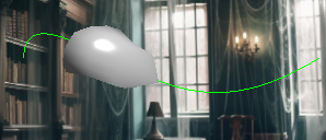
Player Control: The control scheme is simple and direct. The player’s camera is fixed, looking straight ahead.

• A/D Keys: Control the horizontal position of the sword.
• Mouse X/Y: Control the sword’s roll and vertical position, respectively.

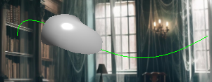
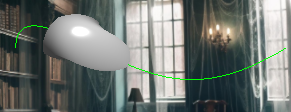
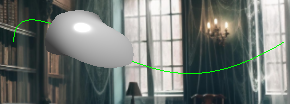
The Slice Animation: When the left mouse button is clicked, we trigger a pre-scripted animation that takes over the sword’s transform for a fraction of a second. We found that a simple linear thrust felt robotic. To make it look natural, we combined three motions, all driven by a smooth sine wave for easing:

1. Forward Thrust: The sword lunges forward into the scene.
2. Downward Dip: It follows a slight arc, dipping down as it thrusts, simulating the motion of a real arm.
3. Pivoted Pitch: This was the most crucial detail. Instead of the whole sword rotating, we made the blade “lean forward” by rotating it around a pivot point located at the handle. This was achieved by finding the pivot’s coordinate in the model’s local space and applying a Translate -> Rotate -> Inverse Translate transformation sequence. This gives the impression that the handle stays stable while the blade does the cutting work.

The actual slice logic is triggered at the very peak of this animation, ensuring the cut happens at the moment of maximum extension.

Adding the juice

CPU Logic: The CPU is responsible for the particle physics. Each frame, it loops through active particles, applies gravity to their velocity, updates their position, and decreases their lifetime.

GPU Rendering: We upload the position, color, and size of every active particle to a buffer in a single batch. Then we call instanced rendering (glDrawArraysInstanced) to draw all active particles efficiently in one call, with each instance using its own position, color, and size.

The number of particles at each moment is not higher than 15000. Therefore, we decided to not use compute shaders and stick to a simpler solution.

Basic Physics

Once an object is sliced into two new pieces, they shouldn’t just hang in the air. We needed a physics system to make them react realistically. We built a simple but effective system from the ground up.

• RigidBody Component: We created a RigidBody class that can be attached to any GameObject. It stores physical properties like mass, velocity (linear and angular), and accumulators for force and torque.
• PhysicsEngine: This central system manages a list of all active rigid bodies. In its update(deltaTime) loop, it performs two key steps:
  1. It applies a constant downward gravitational force to every object.
  2. It updates each object’s position based on its velocity, and its rotation based on its angular velocity.
• Applying Slice Forces: The most important part was making the cut feel impactful. When the SliceManager successfully creates two new pieces, it immediately applies two types of forces to their new RigidBody components:
  1. Separation Force: A force is applied along the plane’s normal, pushing the two halves directly away from each other.
  2. Follow-Through Force: A larger force is applied in the direction of the sword’s slice (the blade’s forward-facing “blue axis”). This gives the pieces momentum and makes it look like the sword’s energy was transferred to them.
  3. Torque: A small, random torque is also applied to each piece to give them a natural-looking tumble as they fly apart.

Gameplay Structure – Game Modes and Spawning

An enum was introduced to manage the current state (FRUIT_MODE or DUMMY_MODE). Pressing the ‘M’ key now switches between these modes, cleans up old objects and prepares the new environment.

• Fruit Mode: every 5 seconds, a fruit (randomly chosen between watermelon, apple and banana) is thrown into the scene.
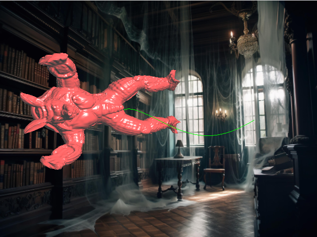
• Dummy Mode: a static humanoid model in the centre of the scene.

Also, independent from the game mode, you can stop the physics of the objects (so that they stay static) and try to slice a fruit/dummy in several directions at once.

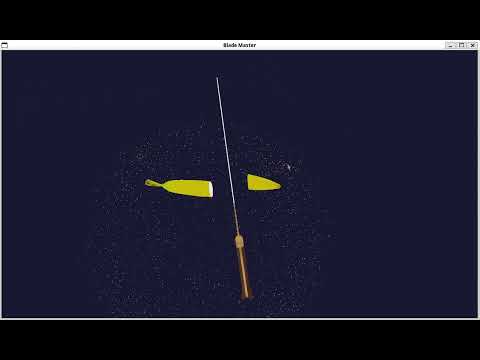
Please see our demo video below:

Murat Şengül & Omar Afandi

Hello again, dear graphics enjoyers!

This post details my approach to the “Particle Magic” assignment for CENG469 Computer Graphics II. The objective was to develop an OpenGL application capable of simulating a large number of points—up to one million—whose movements are influenced by user-configurable gravitational attractors. A key requirement was the use of compute shaders for updating particle states efficiently.

Architectural Overview

In contrast to the previous homeworks, I adopted an OOP methodology this time. This involved refactoring the initial code into several distinct classes, each with specific responsibilities:

• InputHandler: Processes keyboard and mouse inputs, translating them into actions within the Application and SceneManager.

• Application: Serves as the central orchestrator, managing the GLFW window, the main application loop, and the interaction between other components.

• ShaderManager: Handles the loading, compilation, and linking of all GLSL shader programs (vertex, fragment, and compute).

• ParticleSystem: Manages the core particle data, including positions, velocities, and ages. It interfaces directly with the compute shader for state updates and handles the rendering of particles.

• SceneManager: Oversees the simulation environment, including the collection of gravitational attractors, the particle spawn origin, simulation speed (delta time scaling), and user interaction modes.

• TextRenderer: Responsible for rendering on-screen text for the user interface, utilizing the FreeType library.

Core Simulation: Particle Behavior and Compute Shader Mechanics

Each particle maintains a state comprising its position (glm::vec3), velocity (glm::vec3), and current age (float). The age attribute decrements over time, and upon reaching zero, the particle is “respawned.”

Gravitational attractors, defined by their position and mass (float), exert forces on the particles. The magnitude of this force is proportional to the attractor’s mass. The simulation is initialized with a default set of attractors, and users can add or remove attractors dynamically.

The computational core of the simulation resides in the compute shader. For each frame, the compute shader performs the following operations for every active particle:

1. State Retrieval: The particle’s current position, velocity, age, and its initial maximum age (used for normalization) are read from a Shader Storage Buffer Object (SSBO).
2. Gravitational Force Accumulation:
   • A net force vector for the particle is initialized to zero.
   • The shader iterates through all active attractors. For each attractor:
     • The vector from the particle to the attractor (Direction = AttractorPosition - ParticlePosition) is calculated.
     • The squared distance (DistanceSquared) is computed.
     • The magnitude of the gravitational force is determined using a formula: ForceMagnitude = (GravitationalConstant * AttractorMass) / DistanceSquared. The particle mass is implicitly assumed to be 1.
     • The force vector from the current attractor is normalize(Direction) * ForceMagnitude.
     • This vector is added to the particle’s net force accumulator.
3. Velocity Update:
   • The accumulated net force is treated as acceleration (assuming unit mass for particles: Acceleration = NetForce).
   • The particle’s velocity is updated: newVelocity = oldVelocity + Acceleration * deltaTime.
   • A damping factor (e.g., newVelocity *= 0.995f) can be applied to gradually reduce velocity, contributing to simulation stability and visual style. Commented out in the version I submitted.
   • The velocity is capped at a MAX_SPEED to prevent particles from becoming uncontrollably fast.
4. Position Update:
   • The particle’s position is updated based on its new velocity: newPosition = oldPosition + newVelocity * deltaTime.
5. Age Progression and Respawn Logic:
   • The particle’s age is decremented: currentAge -= deltaTime.
   • If currentAge <= 0.0f:
     • The particle’s position is reset to the current particleOrigin (a user-controllable point).
     • Its currentAge is reset, often to its initial_max_age (which can be randomized slightly upon each respawn for variation).
     • A new initial velocity is assigned. This is a key area for artistic control, allowing for various emission patterns.
6. State Storage: The updated position, velocity, and age are written back to the particle’s entry in the SSBO.

Conclusion

It was a very fun experience and a great opportunity to enhance my portfolio with such a nice project. Many thanks to Oğuz Hocam and Kadir Hocam. I’m thrilled to apply this knowledge to create various visual effects in my future projects. Thanks for reading!

Hello again, dear Graphics enjoyers! The mission for Homework 2 was to build a renderer capable of handling HDR cubemaps, deferred shading for our armadillo friend, motion blur, and finally, tone mapping to bring it all to our LDR screens. It’s been a fantastic learning experience with a multi-stage pipeline!

Control Keys

Camera: Middle Mouse Button + Drag

Exposure: Page Up/Down

Key value: Up/Down

Gamma on/off: g

Tone-mapped and Gamma-corrected mode: 0

Cube-only mode: 1

Positions mode: 2

Normals mode: 3

Deferred rendering mode: 4

Composite mode: 5

Composite and Motion Blur mode: 6

HDR Skybox

First, I set up an HDR cubemap to create a realistic environment. The brightness of this skybox is adjustable using an exposure control (Page Up/Down keys).

Deferred Shading

Instead of traditional forward rendering, we implement deferred rendering in this homework.

Geometry Pass

The armadillo’s world-space positions and normals are rendered into off-screen textures (the G-Buffer). Modes ‘2’ and ‘3’ let me visualize these G-Buffer outputs:

Lighting Pass

A full-screen quad then uses this G-Buffer data to calculate Blinn-Phong lighting for the armadillo. I used three different point lights.

Compositing

The lit armadillo is then blended with the previously rendered skybox. A tricky bit here was ensuring background pixels (where the armadillo isn’t) correctly became transparent to show the skybox. This involved fixing how background normals were handled in the lighting shader.

Motion Blur

I implemented a screen-space box blur that activates based on camera rotation speed. The blur strength ramps up with faster mouse movements and gradually fades when the camera stops. The output of this pass also stores the log-luminance of each pixel in its alpha channel, ready for tone mapping.

Gamma Correction

I’ve also added a gamma correction step, which can be toggled with the ‘G’ key.

Here gamma correction is disabled:

Here gamma correction is enabled:

Tone Mapping

The final stage is tone mapping, specifically Reinhard global tone mapping, to convert the HDR image (from the motion blur pass) into something viewable on a standard display. This involves calculating the log-average luminance of the scene (by generating mipmaps from the motion blur texture’s alpha channel) and using it with an adjustable keyValue (Up/Down arrow keys).

However, this is where I’ve hit a wall. The tone-mapped output currently looks quite “strange.” The most noticeable issue is that the scene’s brightness and contrast shift significantly when the camera is moving (even when motion blur is disabled). When the camera stops, the image settles into a more stable state.

Moreover, for some reason armadillo is not displayed in this mode on inek machines.

Text Rendering

Conclusion

It was indeed a very rewarding experience. Many thanks to Oğuz Hocam for this wonderful learning opportunity.

Thanks for reading, and see you in the upcoming homework!

Welcome, dear Computer Graphics enjoyers!

In this blog, I will talk about some details of my implementation for CENG469 Computer Graphics II homework and the challenges I faced.

Curved Path Generation

I decided to start with this part as it seemed to be the easiest one. I implemented BezierCurve class. Throughout the whole program, I keep one global instance of BezierCurve class, which is instantiated with hardcoded control points at the beginning of the program. Each frame the t parameter of the curve is increased by a hardcoded delta value. When the end of the curve is reached, we update the control points of the BezierCurve class instance with the newly generated random control points, ensuring that the path is C1 continuous and stays in the scene bounds. The range of x, y and z coordinates, in which the control points are generated, was found experimentally.

In the later stage of implementation – when I already aligned the model to the path – I faced the following problem: despite being C1 continuous, the path didn’t feel smooth. I minimized this by regenerating control points which are too close to each other.

Alignment and Rolling

The part I continued with was making Armadillo follow the path.

At each frame, Armadillo is translated by the current point of the curve. Then I aligned the gaze of Armadillo with the current tangent of the curve as described in the specification 11 of the homework text. However, I faced the following problem: while following the path, Armadillo gradually “falls” to one side:

The interesting part is that this issue wasn’t present when I was calculating right vector as a cross-product of the tangent and the world’s up, in contrast with calculating right as a cross-product of the tangent and the previous point’s up (the up vector calculated in the previous frame). Neither was this solution suitable as Armadillo was often flipping, while following the path.

I decided to combine these two solutions: using world’s up by default and prevUp when the tangent and the world’s up are close to being parallel. This approach seemed to resolve the issue. Nevertheless, the ghost didn’t have this problem, so I used only prevUp in the final implementation.

Alternating rolling motion was done using glm’s built-in quaternions.

Ghost

I designed ghost using five surfaces: four identical rotated surfaces and one concave bottom-surface (no holes in the mesh). Here are screenshots from MATLAB:

Each surface was rendered separately using the pipeline implemented in the template code.

s=t=1

s=t=2

s=t=3

s=t=5

s=t=10

s=t=25

s=t=50

s=t=100

Here is the final video showing all keyboard interactions:

Conclusion

In overall, it was a very satisfying experience. Many thanks to Oğuz Hocam and Kadir Hocam for such a great learning opportunity. The template code was very helpful.

Thanks for reading and see you in the upcoming homework!

Welcome to METU Blog Service. This is your first post. Edit or delete it, then start blogging!