Methodology
During this analysis, two methods were used to extract the inverse response curves out of two series of pre-captured sequences with known exposures and one sequence captured with my own Galaxy S26 FE device, which also had its exposures recorded.
Debevec & Malik - As used directly through its OpenCV library, it solves for the log inverse response through a 256 value free table. Sampled pixels are then used to compute least squares error, where a smoothness term is then added, while the hat weight w(z) counts the values near 0 and 255 less:


Mitsunaga & Nayar - Like it is integrated as in the PICCANTE implementation, this one computes the inverse response as a low order polynomial with the constraint of f(1) = 1. There, the same pixels seen in two consecutive images should differ by the exposure ratio R_q, while the error is built on that:


So, while Debevec utilizes 256 plus P unknown values, MN uses only N of them. MN also has the ability to recalculate the exposure ratios and pick the best degrees by itself. All in all, this difference in number of unknowns can be seen to explain many of the results below.
Libraries
| Method | Implementation | Version |
|---|---|---|
| Debevec & Malik | OpenCV cv2.createCalibrateDebevec - https://github.com/opencv/opencv | opencv-python 5.0.0.93 |
| Mitsunaga & Nayar | PICCANTE MitsunagaNayar - https://github.com/banterle/piccante | commit 9a2bbf0 |
For Debevec, implementation was already ready through OpenCV with Python. Mitsunaga-Nayar, on the other hand, was not in OpenCV or any other public Python package, so I picked PICCANTE's CPP implementation from GitHub. To integrate, I only used a wrapper for Python to call on its own end and handle the main operations and presentation elements through Python.
I used the parameters:
- Debevec - 70 samples on a grid and λ = 10 as per OpenCV default parameters
- MN - best degree out of 1...3 and alpha = 0.04, with ratio update off (PICCANTE defaults)
Difficulties I faced during the integration of these libraries were:
- PICCANTE crash - where the latest commit was emptying the sample array before trying to use it. So, I used the commit before that.
- Compiling - faced an issue of missing "stb" headers, then turned them off with the library's own "-DPIC_STB_DISABLE" switch as Python is the side that handles the reading of the images here.
- Negative values - the MN polynomial could reach below zero at the darker ends while the merge was trying to take a logarithm of it. I replaced such values with very small numbers instead.
- sRGB formula - while the assignment pdf was stating the usage of 0.05 value here, related sources were instead using 0.055 as a standard to keep the curve continuous and ending at the value 1.
Finally, Evaluation Metrics
- The virtual camera response was known as sRGB or linear and its exposures were noted to be used like they double at each step.
- Due to the curves having an arbitrary scale, each channel is scale-fitted with Z = 20-230 and then, compared with an RMSE of over Z = 5-250.
- "Real camera results" had no applicable ground truth, so for hem, I checked to see if a curve is positive and positively scaling at all times.
Virtual Camera Results
RMSE using the default parameters:
| Sequence | Debevec-Malik (OpenCV) | Mitsunaga-Nayar (PICCANTE) |
|---|---|---|
| srgb | 0.0500 | 0.0025 |
| linear | 0.0323 | 0.0007 |
| noise25 | 0.2056 | 0.0031 |
| noise50 | 0.1634 | 0.0046 |
| noise100 | 0.1756 | 0.0492 |
| noise150 | 0.2523 | 0.0730 |
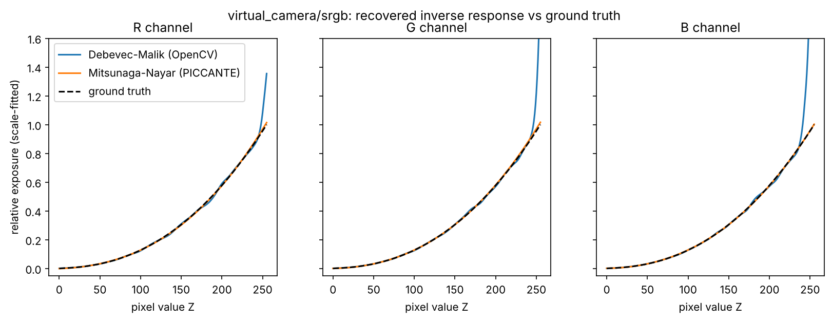
Figure 1 - sRGB virtual camera - both results and the actual inverse sRGB curve.
These initial results show MN to be the clearly more accurate result. The curve fits a smooth, gamma-like structure well enough and hits the degree 1 as required for the linear camera (reaches up to 3 for sRGB). Debevec's results, on the other hand, presents small amounts of flickering while the top end, above z = 240, shoots up by a clear margin.
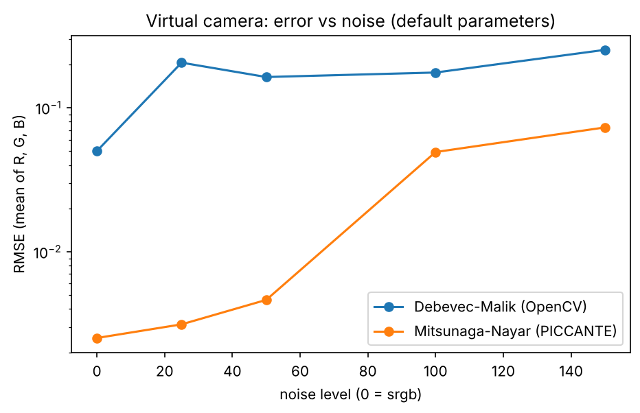
Figure 2 - error against noise level.
The observed gap grows even bigger with the introduction of noise into the fold. Debevec hat weight still gives some weight to nearly saturated pixels, while MN's "alpha" parameter drops the samples close to 0 and 255 entirely, which seems to make the difference here as we can see in later parts.
Real Camera Results
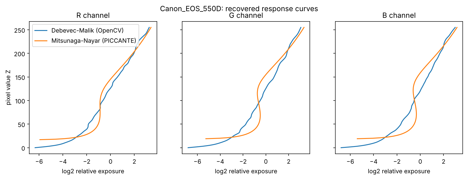
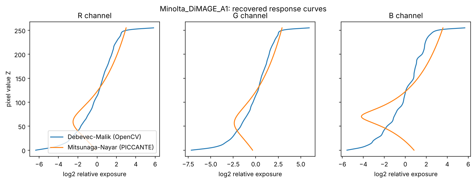
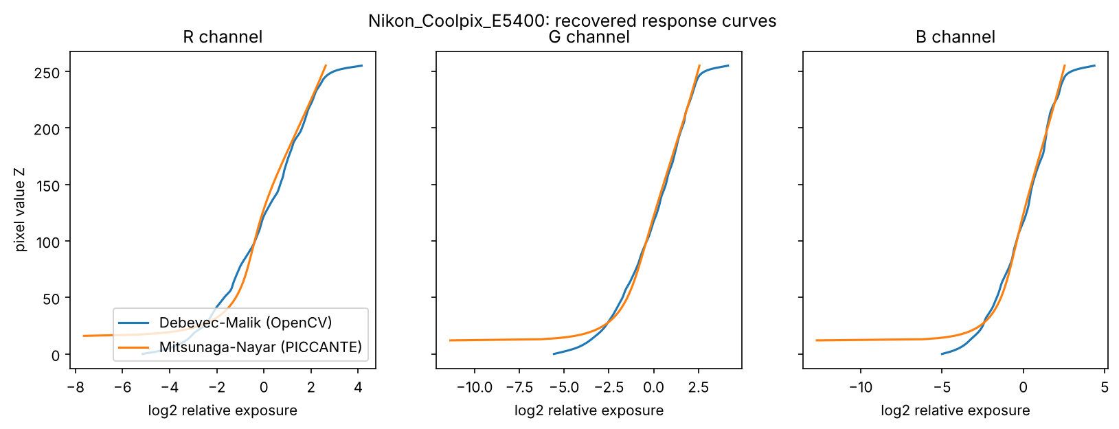
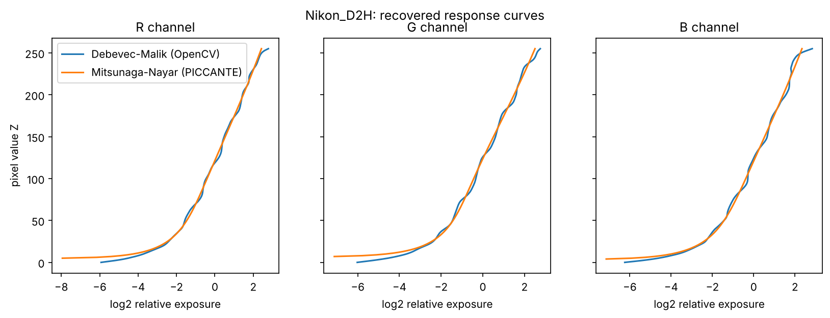
Figure 3 - recovered curves of all four real cameras.
| Camera | Debevec-Malik - Decreasing Steps R/G/B | Mitsunaga-Nayar: Degree | Mitsunaga-Nayar - Decreasing Steps R/G/B | Mitsunaga-Nayar: Values ≤ 0 R/G/B |
|---|---|---|---|---|
| Canon EOS 550D | 3/0/0 | 3 | 17/46/50 | 17/19/19 |
| Minolta DiMAGE A1 | 0/0/0 | 2 | 59/56/70 | 0/0/0 |
| Nikon Coolpix E5400 | 0/0/0 | 3 | 0/0/0 | 16/12/12 |
| Nikon D2H | 0/0/5 | 3 | 0/0/0 | 5/7/4 |
As seen from the results above: On Coolpix and D2H, both methods agree quite well, which also shows that the 2^EV exposures used for D2H were correctly selected. For Canon and Minolta, however, MN's curve bends backwards in the shadows, while Debevec's curves stay plausible for all four settings.
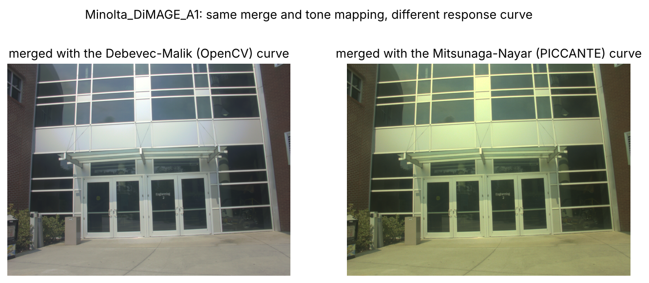
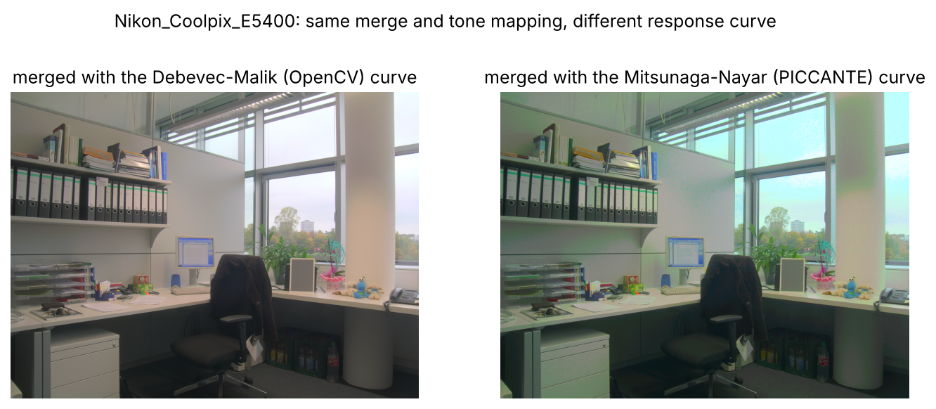
Figure 4 - same merge and tone mapping with different curves.
Results can be observed similarly in the HDR results as seen above again. Coloring of Debevec's results remain natural, while the saturation seems off with visible yellow and cyan tints being discernable.
Parameter-Variant Testing
| Method | Parameter | Definition | Default |
|---|---|---|---|
| Debevec-Malik | lambda | weight of the smoothness term | 10 |
| Debevec-Malik | samples | number of pixel positions used | 70 |
| Mitsunaga-Nayar | polynomial_degree | a fixed degree, or the best one out of 1..N | best out of 1..3 |
| Mitsunaga-Nayar | alpha | pixels outside [alpha, 1-alpha] are dropped | 0.04 |
| Mitsunaga-Nayar | computeRatios | re-estimates the exposure ratios | off |
Parameter sweeps were done only with the virtual camera, as that is only where the errors could be recorded.
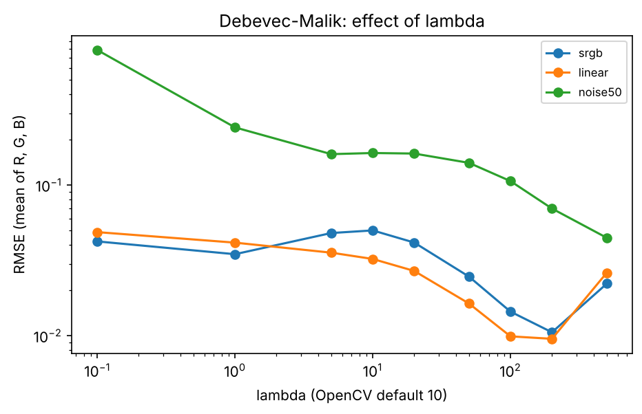
- Debevec lambda - the default value of 10 was too low to minimize the error in the tested sequences. With lambda around 100-200, the srgb error almost drops by %80, while going higher than that over-smooths the curve. One exception is with noise (noise50) though where even higher lambda choices can further improve the results.
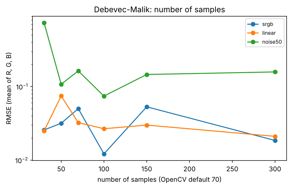
- Debevec samples - in this case, more or less samples didn't amount to better or worse results consistently. Running time, however, saw a significant increase with an increased number of samples.
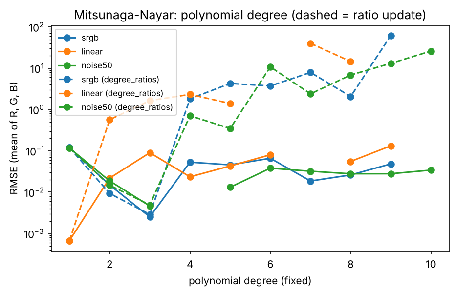
- MN degree - the best degree appears to be 3 for srgb and 1 for linear. Higher degrees only produce worse results and can be observed to cause the curve to oscillate on the real camera sequences. So, the default setting is satisfactory.
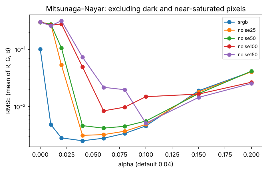
- MN alpha - apparently, this was the most important parameter of them all. With alpha = 0, MN fails with every single sequence. As noise increases, a larger alpha is noted to be beneficial overall:
- 0.04 is enough up to noise50
- noise100 needs 0.06
- noise150 needs 0.1
- On the real cameras, alpha = 0.1 makes Minolta's curve turn fully monotonic.
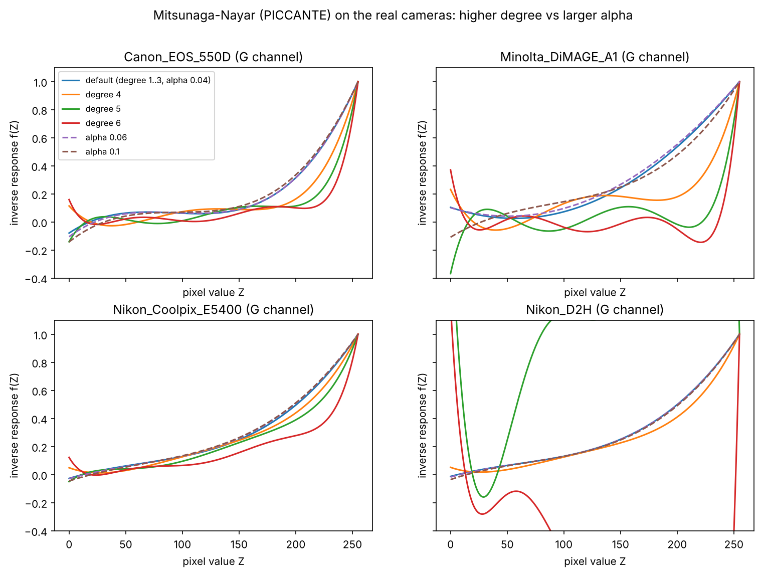
- MN ratio update - this one didn't help and appears to diverge at higher degrees. Since the true ratios are already known in our case, re-estimating only worsens the results.
Running Durations
Following time records were obtained for the curve recoveries, with the following environment: Intel Core i7-11800H, Windows 11.
| Sequence | Images | Size | Debevec-Malik (s) | Mitsunaga-Nayar (s) | Debevec / MN |
|---|---|---|---|---|---|
| Canon EOS 550D | 9 | 5184x3456 | 2.365 | 1.210 | 2.0 |
| Minolta DiMAGE A1 | 13 | 1600x1200 | 3.364 | 0.184 | 18.2 |
| Nikon Coolpix E5400 | 16 | 2592x1944 | 3.460 | 0.633 | 5.5 |
| Nikon D2H | 9 | 2464x1632 | 2.830 | 0.267 | 10.6 |
| virtual: srgb | 9 | 1024x1024 | 2.489 | 0.072 | 34.6 |
| virtual: linear | 7 | 1024x1024 | 1.990 | 0.057 | 34.7 |
| virtual: noise25 | 9 | 1024x1024 | 2.527 | 0.072 | 34.9 |
| virtual: noise50 | 9 | 1024x1024 | 2.442 | 0.074 | 33.2 |
| virtual: noise100 | 9 | 1024x1024 | 2.447 | 0.074 | 33.1 |
| virtual: noise150 | 9 | 1024x1024 | 2.411 | 0.074 | 32.6 |
| Samsung Galaxy S26 FE | 10 | 3000x4000 | 2.724 | 0.929 | 2.9 |
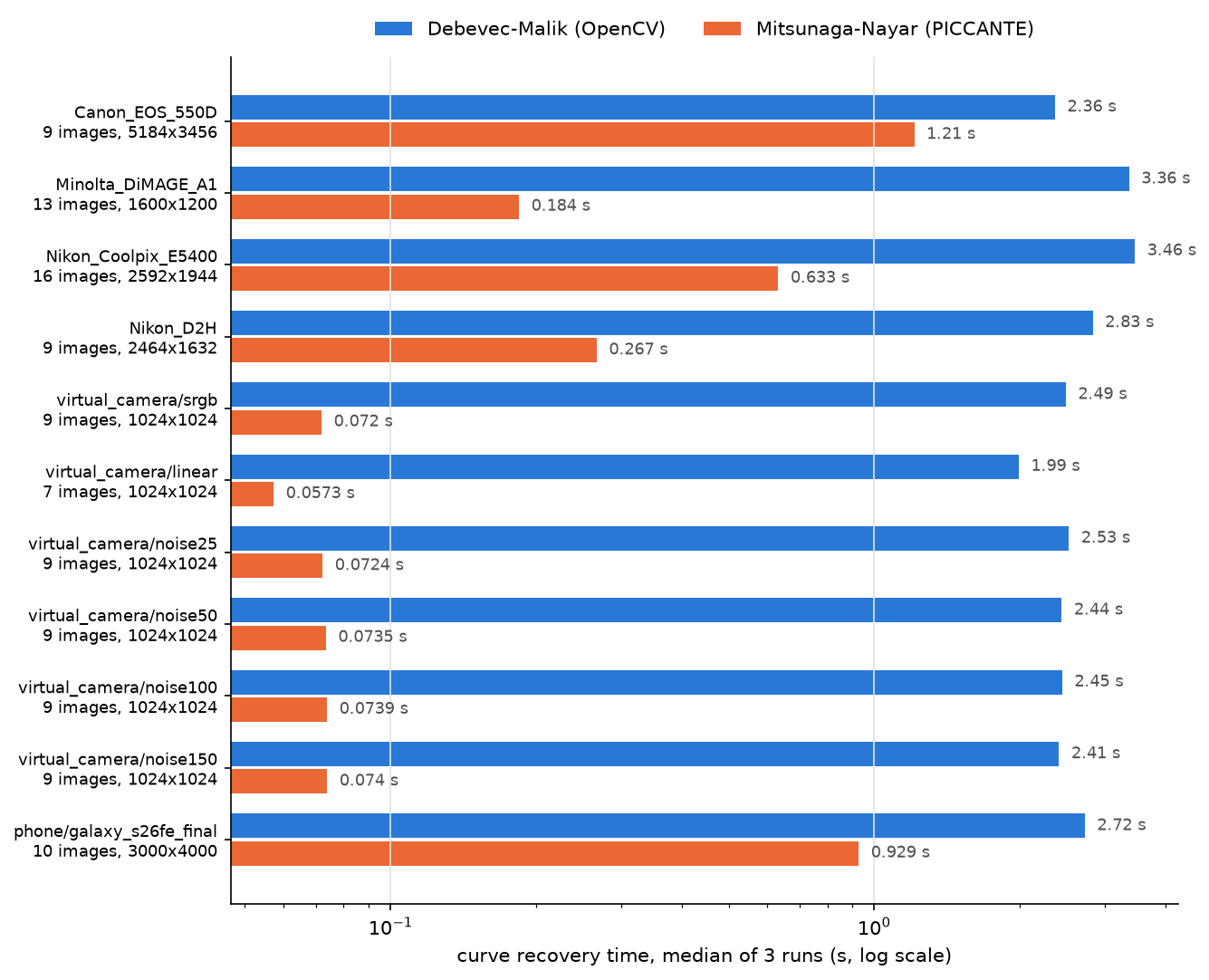
MN appears to be 2 to 35 times faster in all sequences, while Debevec's runtime is independent of the image size, since its cost comes from a larger linear system that relies on the number of samples and image count instead. MN, on the other hand, extracts the histogram of each image and then solves a very small linear system, thus resulting in its duration growing with each added pixel.
My Own Capture
Capture details
- Device - Samsung Galaxy S26 FE, main camera, fixed aperture f/1.8
- App - native camera app in Pro mode, JPEG only
- Fixed manually - ISO 50, white balance and focus
- Varied - shutter speed only, from 1/500 s to 1 s, each step roughly doubling the previous one (10 shots)
- Scene - indoors, lit only by daylight coming through an open door and a glass bottle on a table with a mirror behind it, which looks towards something else
- Handheld, no additional equipment were available for use. All 10 shots taken within 52 seconds, with only very slight shifts between frames.
- EXIF exposure times matched the values set by hand and used directly.
All in all, finding a place worthy of capture was kind of hard. Any outside attempts were constantly being broken of by envrionmental changes, natural motions, people passing by etc. So, I decided to capture under an environment with natural lighting, on a target that is worthy of praise just as nature itself: A 1 liter glass bottle of an anonymous brand of mineral water.
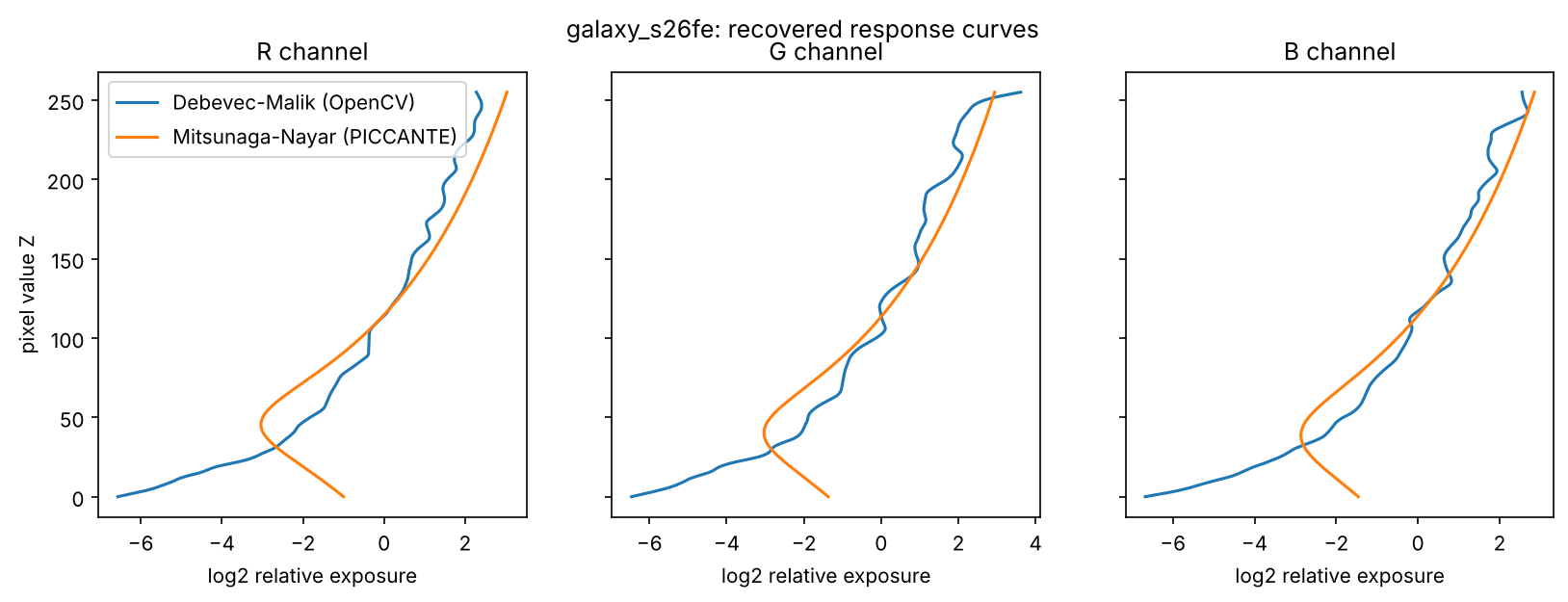
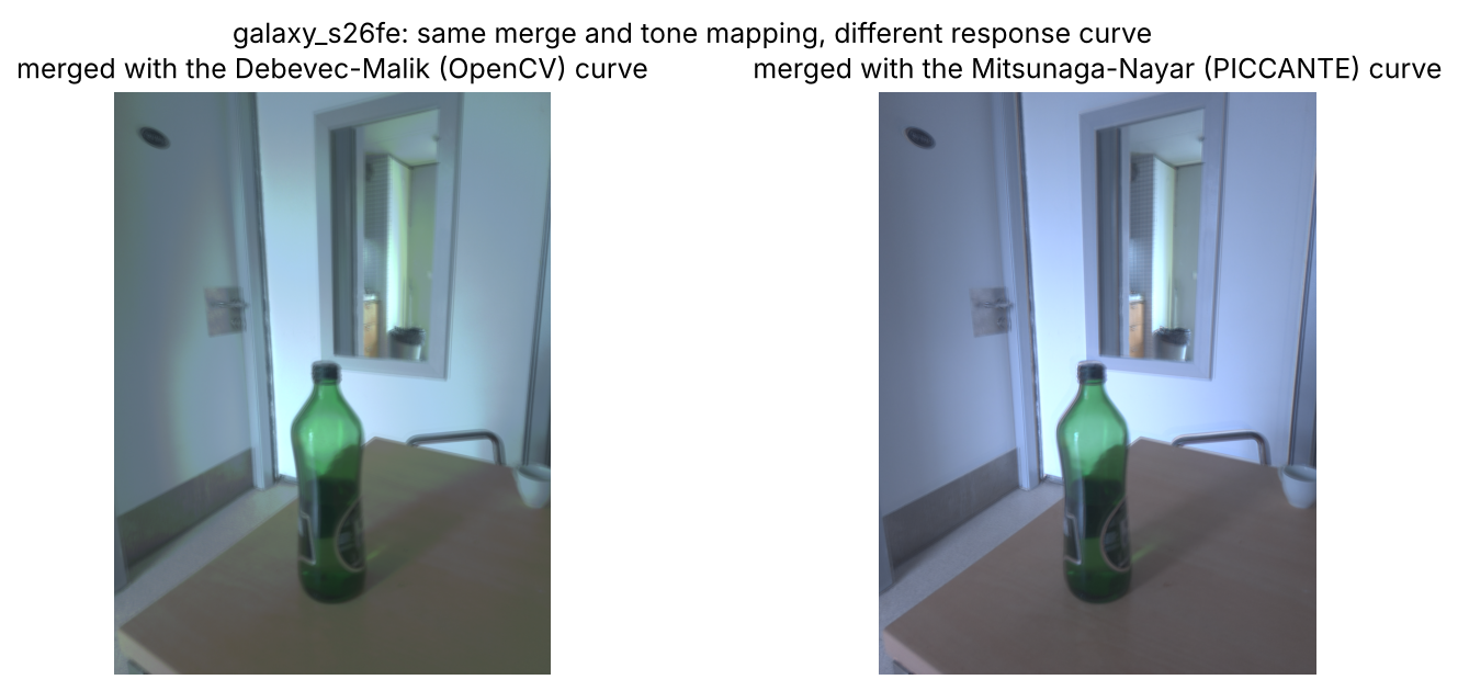
Figure 5 - Galaxy S26 FE - recovered curves and HDR previews.
| Method | Degree | Decreasing Steps R/G/B | Values ≤ 0 R/G/B | Time (s) |
|---|---|---|---|---|
| Debevec-Malik (OpenCV) | - | 32/40/47 | 0/0/0 | 2.724 |
| Mitsunaga-Nayar (PICCANTE) | 2 | 45/40/39 | 0/0/0 | 0.929 |
Final results show the middle tones and highlights to be well handled, where the derived response curve is smooth and gamma-like. However, they appear to have split in darker areas, where MN bends backwards just like a few previous examples; while Debevec stays monotonic with minor flickers above Z = 90. This supports the previously found results of the default lambda bening too low to handle those parts. Outside of these, color balance is more proper on both ends while each of them a have a slight bias in their tint to different ends. No ghosting or similar artifacts are observed either.
An issue to note from my own perspective would be the large amount of decreasing steps against the real camera scenarios (for Debevec, at least). I couldn't quite pinpoint the reason for this, but the difference in how clean each curve is may be related to the weakness of handheld capture.
Conclusion
- Accuracy - when the ground truth is known, MN appears to be much more accurate (0.0025 against 0.0500 on srgb).
- Robustness - on the real cameras, Debevec is the more reliable one, as MN's default curves are not monotonic in the shadows on two cameras and on my phone.
- Speed - MN is 2 to 35 times faster.
- Critical parameter based on findings - lambda for Debevec, as the default value is too low, and alpha for MN as it is better for it to grow with noise.
Nothing can be said about the differences of individual implementations of the two methods, as only OpenCV and PICCANTE implementations are tested and no testing is done with respect to other similar ones to evaluate their success.
For my own use with my own phone's captures, I would probably make my choice on the perceivable difference instead of relying on numeric evaluation. Debevec has a discoloring tint on its subjects, so my pick would be MN most of the time. Though, for professional settings and different purposes of capture, Debevec could still come up better for some people.
Sources
- P. E. Debevec, J. Malik, "Recovering High Dynamic Range Radiance Maps from Photographs", SIGGRAPH 1997.
- T. Mitsunaga, S. K. Nayar, "Radiometric Self Calibration", CVPR 1999.
- E. Reinhard et al., "Photographic Tone Reproduction for Digital Images", SIGGRAPH 2002.
- OpenCV (Apache-2.0): https://github.com/opencv/opencv
- PICCANTE (MPL-2.0), F. Banterle et al.: https://github.com/banterle/piccante (commit 9a2bbf0)
Leave a Reply