I decided to start by improving the performance of ray tracer since I hadn’t made any work in that aspect. Please keep in mind that the measurements were taken on a M3 Max CPU with 16 cores. Also, each new measurement uses all of the optimizations that came before it.
My ray tracer was single threaded, so the easiest performance gain seemed to be adding multithreading. My implementation for this is simple. The image gets broken up into 50×50 regions that get pushed into a queue, then n(number of cores) worker threads spawn. These threads pop a region from the queue with concurrency protection, then start rendering the region. This loop continues for each worker until the queue is empty. After that, all the threads join the main thread, then the image gets written as before. Here’s a worker thread’s loop:
void renderTask(
std::queue<RenderRegion> ®ions,
std::mutex& regionsMutex,
const Camera& camera,
Pixel* buf
) {
while (true) {
regionsMutex.lock();
if (regions.empty()) {
regionsMutex.unlock();
return;
}
auto region = regions.front();
regions.pop();
regionsMutex.unlock();
renderChunk(camera, buf, region);
}
}
| Scene | Single-threaded | Multi-threaded |
| bunny_with_plane | 58000~ ms | 5000~ ms |
| simple | 40~ ms | 20~ ms |
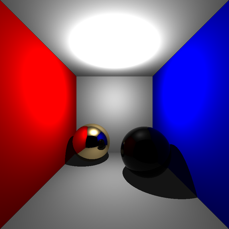
| cornellbox_recursive | 140~ ms | 35~ ms |
| bunny | 5400~ms | 550~ ms |
Multi-threading improved the performance dramatically, especially in larger scenes. For further performence improvement, I decided to implement back-face culling. I simply added an if statement to the mesh and triangle intersections:
if (attemptCull && glm::dot(ray.direction, face.normal) > 0) {
    return false;
}
Back-face culling improved performance significantly in scenes with large meshes.
| Scene | Without Back-face Culling | With Back-face Culling |
| bunny | 550~ ms | 430~ ms |
| bunny_with_plane | 5000~ ms | 4000~ ms |
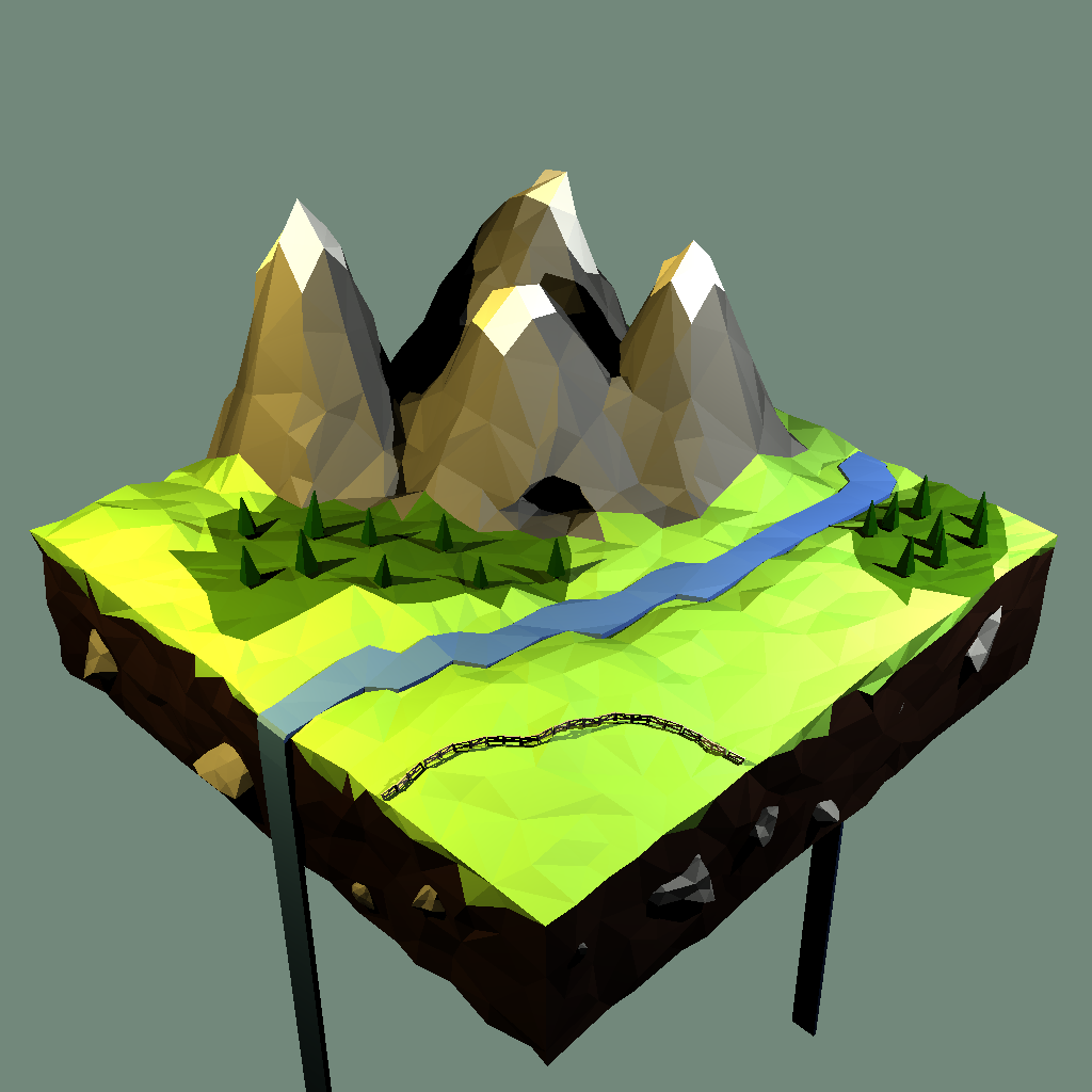
| low_poly_smooth | 3500~ ms | 2800~ ms |
My next step was to implement a BVH. I started by adding a simple AABB class so that I can intersect rays with it.
class AABB {
public:
glm::vec3 axesMin;
glm::vec3 axesMax;

bool hitRay(const Ray& ray) const {
    float t1Max = std::numeric_limits<float>::min();
    float t2Min = std::numeric_limits<float>::max();

    for (int axis = 0; axis < 3; ++axis) {
        auto oneOverRayDirection = 1.0f / ray.direction[axis];
        auto t1 = (axesMin[axis] - ray.origin[axis]) * oneOverRayDirection;
        auto t2 = (axesMax[axis] - ray.origin[axis]) * oneOverRayDirection;

        if (oneOverRayDirection < 0.0f) {
            auto temp = t1;
            t1=t2;
            t2=temp;
        }

        t1Max = t1 > t1Max ? t1 : t1Max;
        t2Min = t2 < t2Min ? t2 : t2Min;
    }

    if (t1Max > t2Min) {
        return false;
    }

    return true;
}
};
Then, my next step was to compute the bounding boxes of each triangle, sphere, and mesh. For this purpose, I added an instance of my class AABB to my base class Shape. After that, I added the virtual method computeBoundingBox to Shape, and I implemented it for each type of shape except planes.
I had initially planned to continue with the declaration of the BVH class, then BVH tree construction but I got a little sidetracked because I got curious. I added a single if statement to my naive ray intersection method, under the mesh intersections:
if (!mesh.boundingBox.hitRay(ray)) continue;I took measurements of scenes with large meshes.
| Scene | Without Mesh Bounding Box Check | With Mesh Bounding Box Check |
| bunny | 430~ ms | 200~ ms |
| bunny_with_plane | 4000~ ms | 1500~ ms |
| low_poly_smooth | 2800~ ms | 870~ ms |
With a simple bounding box check, large meshes could now be rendered much faster than before. I carried on by defining the BVHNode class including the traversal method.
class BVHNode {
public:
    enum NodeType {
        LEAF,
        INTERNAL
    };

    NodeType nodeType;

    // INTERNAL
    AABB boundingBox;
    std::unique_ptr<BVHNode> left;
    std::unique_ptr<BVHNode> right;
    // LEAF
    void* object;

    bool searchNodes(const Ray& ray, std::vector<void*>& hitList) const {
        if (!boundingBox.hitRay(ray)) {
            return false;
        }

        if (nodeType == LEAF) {
            hitList.push_back(object);
            return true;
        }

        bool hitLeft = left!=nullptr && left->searchNodes(ray, hitList);
        bool hitRight = right!=nullptr && right->searchNodes(ray, hitList);

        return hitLeft || hitRight;
    }
};
Then It was straightforward to write the BVH class with a dummy buildTree method.
class BVH {
public:
    std::unique_ptr<BVHNode> root;

    bool hitRay(const Ray& ray, HitInfo& hitInfo) const {
        return root->hitRay(ray, hitInfo, vertices, vertexNormals);
    }

    static BVH buildTree(std::vector<Shape*>& shapes, size_t start, size_t end) {
        BVH result;

        result.root = buildNodes(shapes, start, end);

        return result;
    }
private:
    static std::unique_ptr<BVHNode> buildNodes(std::vector<Shape*>& shapes, size_t start, size_t end) {
        return std::make_unique<BVHNode>();
    }
};
Then, I implemented the tree building method. I won’t put the code here to not clutter up the post, but the algorithm was basically this:
1-) Take the array of objects with an upper and lower bound.
2-) Choose a random axis to split the objects upon.
3-) Sort the objects with respect to the chosen axis. The comparison values used during this sort is the mid point of the bounding boxes of the objects(i.e. equal count heuristic).
4-) Split the sorted array into two equal segments, then recursively call the method again with new upper and lower bounds.
5-) Once the children have been computed, combine their bouing boxes to compute the current node’s bounding box and return the results.
With this under the belt, I measured times again. Unfortunately, the results were pretty much the same as the one before. After inspecting the code a little, I realized that the implementation was not complete for mesh objects. Namely, I was successfully “bringing” the rays to the bounding box of the mesh, but after that, I was calling the naive intersection method to actually intersect with the object which is slow because it iterates through every single face. To fix this, I decided to extend my BVH implementation to support two types of trees, namely outer and inner. Then, I assigned the initial tree as the outer tree, then constructed inner trees with the same algorithm only for meshes.
I tested the performance once again:
| Scene | Without BVH | With BVH |
| bunny | 200~ ms | 15~ ms |
| bunny_with_plane | 1500~ ms | 70~ ms |
| low_poly_smooth | 870~ ms | 160~ ms |