Z = f(E · Δt)
In this homework I compared two methods that find f⁻¹ from photos taken with different exposure times:
- Debevec & Malik (1997): It does not assume a formula for the curve. It finds all 256 values of g = ln f⁻¹ by solving one big linear system. There is a smoothness term with a weight λ, so the curve does not become noisy. It needs the exposure times.
- Mitsunaga & Nayar (1999): It assumes f⁻¹ is a polynomial of order N. It only needs to find N+1 coefficients, so it is fast. It can also estimate the exposure ratios, so the exact exposure times are not necessary.
I chose Option 2. I compared two algorithms. For Debevec & Malik I used two different implementations and for Mitsunaga & Nayar one, so there are three versions in total:
| Name | Algorithm | Source |
|---|---|---|
| Debevec (OpenCV) | Debevec & Malik | OpenCV cv2.createCalibrateDebevec (70 samples, λ = 10) |
| Debevec (Piccante) | Debevec & Malik | Piccante HDR library (github.com/banterle/piccante), function gsolve, converted from C++ to Python with the help of an AI assistant (256 samples, λ = 20) |
| Mitsunaga (Piccante) | Mitsunaga & Nayar | Piccante, function MitsunagaNayarClassic, converted from C++ to Python with the help of an AI assistant (order N chosen from 1–3) |
I checked the Python versions by testing them on images with a known response curve (the virtual camera), and they recovered the correct curve.
Some details:
– Sample selection. The Piccante versions choose sample pixels with histograms (the Grossberg–Nayar idea): the brightness order of the pixels is the same in every photo, so the same percentile belongs to the same scene point. OpenCV picks 70 random pixel positions instead.
– Same merging for all. I merged every curve to an HDR image with the same OpenCV function (MergeDebevec) and tone mapped it with the same operator (Reinhard). So the differences in the results come only from the curves.
– My computer: MacBook Air, Apple M4 chip, 24 GB RAM, Python 3.9, NumPy 2.0, OpenCV 5.0.
Metrics
- log-RMSE: used when the true curve is known (virtual camera). It is the difference between my curve and the true curve in log scale. Lower is better.
- Consistency error (in stops): used for real cameras, because there the true curve is unknown. If the curve is correct, every photo gives the same light value for the same pixel. I measure how much these values change between photos. 1 stop = 2 times. Lower is better.
Problems
- The first code I found did not work. I first tried the VFX_HDR repository from GitHub. It did not run on my computer: first OpenCV was missing, and the code also uses
np.warnings, which does not exist in new NumPy versions. Its Debevec also uses only 25 pixels, so the curve is not accurate. I decided to use the Piccante library and OpenCV instead. - Setting up Python. The system Python on my Mac did not have OpenCV. I created a virtual environment (
python3 -m venv .venv) and installed the packages withpip install -r requirements.txt. - Wrong EXIF times on the Nikon D2H. See Section 6.2. Because of this, I used “exposure doubles every photo” for all course sequences, as the readme says.
Virtual camera (true curve is known)
The virtual camera images were rendered with the Radiance renderer, and we know their response: srgb, linear, and noise25/50/100/150 (sRGB with more and more noise).
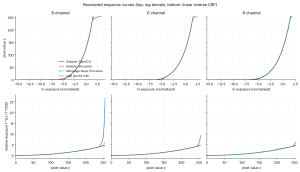
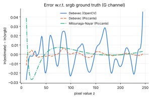
| log-RMSE | Debevec (OpenCV) | Debevec (Piccante) | Mitsunaga (Piccante) |
|---|---|---|---|
| sRGB camera | 0.0239 | 0.0068 | 0.0124 |
| linear camera | 0.0241 | 0.0057 | 0.0027 |
- All three versions find the sRGB curve. Piccante’s Debevec is the closest. OpenCV’s Debevec is good until about z = 240 and then goes up, because its 70 random samples have very few bright pixels.
- For the linear camera, Mitsunaga is the best. A linear curve is exactly a polynomial of order 1, so the model fits it perfectly.
Effect of noise
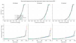
| log-RMSE | Debevec (OpenCV) | Debevec (Piccante) | Mitsunaga (Piccante) |
|---|---|---|---|
| no noise | 0.024 | 0.007 | 0.012 |
| noise 25 | 0.064 | 0.010 | 0.019 |
| noise 50 | 0.100 | 0.019 | 0.092 |
| noise 100 | 0.132 | 0.045 | 0.543 |
| noise 150 | 0.145 | 0.070 | 0.626 |
Debevec gets worse slowly when the noise increases, because the smoothness term keeps the curve smooth. Mitsunaga breaks after noise 50–100: noisy dark pixels pull the polynomial below zero. (I assume the noise sequences have the same sRGB response. The small errors at low noise support this.)
Effect of the parameters
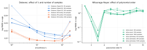
Debevec – λ and number of samples
– Small λ (1) lets the noise into the curve. Big λ (100 or more) makes the curve too flat at the ends. Good values were λ = 5–20 for clean data and λ = 20–50 for the noisy phone images.
– More samples helped OpenCV a lot (50 → 200). Piccante was already good with fewer samples, thanks to the histogram sampling.
– More samples make Debevec slower, because the linear system gets bigger.
Mitsunaga – polynomial order N
– N = 1–2 is too simple and N = 3 was the best. Higher orders (N ≥ 4) gave much worse curves, so the automatic selection between 1 and 3 is a good choice.
– Estimating the exposure ratios gave almost the same result as using the real ratios. The method really does not need exact exposure times when the data is clean.
Real cameras
Sample sequences
All four sequences were run with “exposure doubles every photo” and resized to 1600 pixels.
| Consistency error (stops) | Debevec (OpenCV) | Debevec (Piccante) | Mitsunaga (Piccante) |
|---|---|---|---|
| Canon EOS 550D | 0.168 | 0.167 | 2.288 |
| Minolta DiMAGE A1 | 0.129 | 0.126 | 2.053 |
| Nikon Coolpix E5400 | 0.095 | 0.092 | 1.398 |
| Nikon D2H | 0.110 | 0.107 | 0.161 |
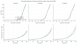
- The two Debevec versions give almost the same curve for every camera.
- Mitsunaga looks fine in the linear plot, but in the log plot it is almost zero below z ≈ 15. So dark pixels get almost no light, and the consistency error becomes very big.
6.2 Nikon D2H: wrong EXIF times
The EXIF data of the D2H says 1/400, 1/320, 1/200, 1/160, 1/100, 1/80, 1/40, 1/20, 1/10 s. The ratios between them are 1.25 and 1.6, but the images clearly get 2 times brighter every time, as the readme says. With the EXIF times, Debevec’s error was 0.259 stops; with doubling it was 0.107. So the EXIF times were wrong, and doubling was the right choice.
7. My phone’s response curve
- Phone: Samsung Galaxy S20 FE
- How I captured: Samsung camera app, Pro mode, JPEG. ISO 500, white balance and focus fixed. I only changed the shutter speed: 1/30, 1/20, 1/10, 1/6, 1/4, 1/2, 1, 2, 4, 10 s (10 photos).
- Scene: In the 10 s photo 84% of the pixels are saturated, in the 1/30 s photo almost none. So all pixel values from 0 to 255 are used.
| Consistency error (stops) | Debevec (OpenCV) | Debevec (Piccante) | Mitsunaga (Piccante) |
|---|---|---|---|
| Samsung S20 FE | 0.129 | 0.128 | 0.771 |
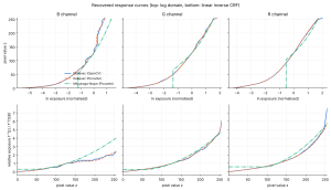
– The two Debevec versions are almost the same, so I take this as my phone’s curve.
– My phone’s curve is not sRGB. When I fit a power function, the exponent is about 1.4 (blue), 1.6 (green) and 1.5 (red). For sRGB it is about 2.2. The phone’s curve is flatter in the middle and bends quickly near 255. I think this is because the phone applies its own tone mapping.
– The blue channel is the hardest. The lamp light is orange, so blue values are low and noisy, and the curve has small steps.
– Mitsunaga failed on the phone. It chose N = 2, the curve went below zero for dark values, and the HDR image got a purple color.
| Debevec (Piccante) | Mitsunaga (Piccante) |
|---|---|
|
|
|


8. Running times
| Sequence | Images | Size | Debevec (OpenCV) | Debevec (Piccante) | Mitsunaga (Piccante) |
|---|---|---|---|---|---|
| Virtual camera sRGB | 9 | 1024×1024 | 26 ms | 168 ms | 69 ms |
| Virtual camera linear | 7 | 1024×1024 | 24 ms | 149 ms | 57 ms |
| Virtual camera noise25 | 9 | 1024×1024 | 27 ms | 157 ms | 59 ms |
| Virtual camera noise50 | 9 | 1024×1024 | 26 ms | 152 ms | 54 ms |
| Virtual camera noise100 | 9 | 1024×1024 | 27 ms | 169 ms | 52 ms |
| Virtual camera noise150 | 9 | 1024×1024 | 27 ms | 155 ms | 53 ms |
| Canon EOS 550D | 9 | 1600×1067 | 28 ms | 213 ms | 113 ms |
| Minolta DiMAGE A1 | 13 | 1600×1200 | 28 ms | 304 ms | 175 ms |
| Nikon Coolpix E5400 | 16 | 1600×1200 | 31 ms | 389 ms | 244 ms |
| Nikon D2H | 9 | 1600×1060 | 27 ms | 206 ms | 108 ms |
| Samsung S20 FE (my phone) | 10 | 1200×1600 | 29 ms | 244 ms | 145 ms |
Times are the median of 3 runs on a MacBook Air (Apple M4, 24 GB RAM), only for finding the curve.
– Debevec (OpenCV) is fast because it uses only 70 samples.
– Debevec (Piccante) is the slowest: 256 samples make a big linear system.
– Mitsunaga solves a very small system. Most of its time goes to making the histograms, so it gets slower with more and bigger images.
9. Conclusion
- With clean data, both algorithms find the true curve. Mitsunaga is the best for the linear camera and it is fast.
- Noise makes the difference. Debevec stays good with noise. Mitsunaga breaks with medium and high noise.
- On all real cameras and my phone, Debevec was the most reliable. One polynomial cannot follow the dark part of real camera curves well.
- Sample selection matters. OpenCV and Piccante solve the same Debevec equations, but the results are a bit different because of the samples.
- EXIF times can be wrong (Nikon D2H).
- My Samsung S20 FE does not have an sRGB curve. Its curve is flatter, with an exponent of about 1.5.
Use of AI: I used an AI assistant (Claude) to convert the Piccante code to Python, help of AI is used for writing the comparison scripts I took the phone photos, ran all experiments on my own computer, checked the results and edited the post.
References
- P. Debevec, J. Malik, “Recovering High Dynamic Range Radiance Maps from Photographs”, SIGGRAPH 1997.
- T. Mitsunaga, S. K. Nayar, “Radiometric Self Calibration”, CVPR 1999.
- F. Banterle et al., Piccante HDR library, https://github.com/banterle/piccante
- OpenCV documentation, https://docs.opencv.org
- M. Grossberg, S. Nayar, “What can be known about the radiometric response from images?”, ECCV 2002.
- E. Reinhard et al., “Photographic Tone Reproduction for Digital Images”, SIGGRAPH 2002.